Tutorial 1: fMRI Data Structures
Goals
To become familiar with core anatomical and functional data formats
To become familiar with core BrainVoyager interfaces, features, and file types
To understand how functional and anatomical scans differ and why accurate co-registration is important
To explore functional data as time series
Relevant Lectures
Basics and Data
Accompanying Data
Background
The goal of these tutorials is to learn practicalities of analyzing brain imaging data. Although the tutorials will later be converted to all the major fMRI analysis packages, we have chosen to use BrainVoyager because it provides an intuitive GUI-based platform that works across operating systems (Mac, PC, Linux) and provides outstanding, straightforward visualization capabilities. Although the goal of the tutorial is not to learn BrainVoyager per se (for that, see BrainVoyager documentation), since we will be using BrainVoyager for tutorials and projects, this tutorial is designed to be an introduction to the fundamental file types (anatomicals and functionals). To complete this tutorial, you can use BrainVoyager 21 on any supported operating system.
The data accompanying this tutorial includes data for an anatomical scan and a functional localizer scan from one participant, along with several other files needed for analysis. Please ensure you are familiar with the localizer and experimental protocols, as outlined in the Experimental Design page. In later tutorials, we will learn how to combine data across scans and participants. However, we will learn the basics with the simplest data set we can have for now.
Basics structure of MRI files
Before getting started, recall that, in most fMRI sessions, an anatomical scan is obtained in addition to any functional scans. In this tutorial, we are using scans for one participant collected at Western University’s Robarts Research Institute Centre for Functional and Metabolic Mapping using a Siemens 3-Tesla Prisma scanner. This scanner records and stores anatomical and functional images using the DICOM digital image format – a standard medical imaging format for MRI data storage and transmission.
An anatomical scan is recorded as a collection of 2D images or slices of the brain. This results in a separate DICOM file for each slice. Using Horos, a free MacOS application for connecting to DICOM servers, we can easily access the DICOM files for our scan. Figure 1 is a rendering of a single DICOM file corresponding to 1 of the 176 sagittal slices of this participant’s anatomical scan. As we can see, this is in fact slice 87 (Im: 87/176), which is slightly lateral to the left-right midline of the brain. This type of scan is called a “T1-weighted” scan in which white matter appears brighter than gray matter and ventricles appear black.
Other information can also be found in the above image, such as slice thickness in mm (1 mm), 2D image size in pixels (224 x 256 pixels), the participant’s anonymized identifier (AQ18), and the name of the study (Culham Psych_9223). If we were to stack the series of anatomical slices, we would have a 3D volume that covered the whole head. Given that the brain anatomy at this coarse scale does not change measurably through a session, only one anatomical volume is collected.

Figure 1. Single 2D anatomical image
Functional scans are also recorded one slice at-a-time and can also be stacked into volumes. However, the angle of the slices – chosen by the experimenters – differed from that of the anatomical slices. Here the slices were tilted off the axial (horizontal) plane. Because functional activity of the brain changes moment-to-moment, we sampled the brain not just once, but repeatedly -- once per second during each functional scan. Another way to phrase this would be to say we collected one volume per second. Note that “volume” can refer to space (specifically our 52 slices that comprise a 3D brain volume) but also to time (340 volumes/scan). Figure 2 is an example of a single functional DICOM file visualized using Horos. This is the set of quasi-axial slices that comprise one volume.
As we can see, this array contains 52 slices of functional data, and is the first volume in a sequence of 340. Together, these 52 slices provide functional data for the entire volume (in this case, the whole brain) within a 1-s period.

Figure 2. Single functional DICOM file
From DICOMs to BrainVoyager Files
Understanding what the raw data looks like straight from the scanner is crucial for understanding how and why BrainVoyager represents fMRI data using other formats. Here we have already converted the data from DICOM to BrainVoyager file types. In this tutorial, we will consider the following file formats:
AMR – Anatomical MR Contain an array of 2D anatomical slices.
VMR – Volumetric MR (Anatomical) Data Set – Three-dimensional data structure for anatomical scans.
FMR – Functional MR Data Set – Simple text file containing information about functional slices; must be partnered with stc files.
STC – Slice Time Course – Functional time series data organized as 2D slice arrays over time
VTC – Volumetric Time Course – Functional time series data organized by 3D volumes over time.
PRT – Stimulation Protocol – Simple text file containing information about experimental stimulus timing over the course of a single run; can be visualized in BrainVoyager.
If you were using other software, you would still have file types that correspond to anatomical scans, functional scans, and the stimulation protocol but the formatting would be different. Increasingly software platforms are moving to a NIfTI (which stands for the Neuroinformatics Technology Initiative), a new standard for file formats and file organization across various software packages. Future versions of the tutorials will provide NIfTI data.
Getting familiar with fMRI files: Instructions
Viewing Anatomical and Functional Slices
1) Open Brainvoyager and click Accept to get started.

2) Click Open , navigate to the folder containing the tutorial data, select AQ18_Anat.amr , and open the file.

The AMR files (AQ18_Anat.amr) are an array of 2D anatomical slices – much like the original functional DICOM files we can view in Horos. Although our analyses will use 3D anatomical files (VMRs) instead, looking at the AMR helps you understand the data as it comes off the scanner and can sometimes be useful for troubleshooting.
Question 1: What slice plane was the data collected in? Hint: If you haven't yet learned anatomical terminology, we recommend you do so now.
3) Next click Open , select AQ18_Loc1-S1R1.fmr , and open the file.
Opening an FMR (text) file also automatically reads in the associated STC (data) files.
The FMR (text) file contains information about the functional scan, including information from the source DICOM files such as the spatial and temporal resolution. Much of this information is displayed in the FMR Properties window. To see the rest, try opening AQ18_Loc1-S1R1.fmr in a text editor like Notepad or TextEdit.
When you open an FMR, you only see the array of slices for the first time point but remember that a function scan involves multiple time points. If you want to see how many time points were collected, look at the fMR Properties window (if you've closed this, you can open it again using File/Document Properties/FMR Properties).

Question 2: How many time points (i.e., volumes) were sampled in this run? Given the number of volumes and the time it took to collect the volume (a measure called the TR), how long in minutes and seconds did this run take? What was the original or "raw" spatial resolution of the functional scan? Are the voxels isotropic or nonisotropic? Give an example of how you might describe the spatial resolution in the methods section of a paper.
Given that functional data is comprised of slice arrays (volumes) over time, we can visualize the 4th dimension (time) by watching the arrays as a movie.
4) Close the FMR Properties window, then select the Options menu, and Time Course Movie. Then click Preload All, wait roughly 5 seconds, and click > to visualize each the functional data over time.
Click the First<->Last button to toogle between the first image that was acquired and the last one.
This is a simple, important step for performing basic quality assurance of your functional data.
Question 3: What might you determine by viewing the Time Course Movie? Do you think this is good quality data? Why or why not?

Viewing Anatomical Volumes
5) Click Open , navigate to the folder containing the tutorial data, select AQ18_Anat.vmr , and open the file.

This VMR provides a 3D view of the anatomical scan generated by "stacking" the 2D slices in a third dimension. The VMR shows three orthogonal planes (sagittal, coronal, and horizontal) centred on a single point (the white crosshairs). Try moving one of the crosshairs to change the view! Note that the views in the other two slice planes change accordingly. It is much easier to get your bearings in a 3D view (the VMR) than the 2D slice arrays (the AMR), which is why we'll be using only the VMRs from this point forward.
So now that we have the anatomical scan in 3D (VMR), we also want the functional scan in 3D. However, recall that the anatomical scans were taken in a different slice plane than the functional scans. Thus, our next step will be to align the functional data with the anatomical scan, so that we can use the participant’s brain anatomy to guide preliminary functional analysis. Although you will likely not have to do these steps in the future tutorials as it will be done for you, it is useful to understand the need for alignment and the possibility that misalignments can occur if bugs or mistakes occur.
Aligning anatomical and functional scans
6) Close the FMR file tab. Look for the 3D Volume Tools window. It may already be on your screen. If it isn’t, click the blue cube to the left of the main window.
a. Then click Full Dialog in the 3D Volume Tools Window.
b. Next click the Coregistration tab, and click the select FMR… button. Select and open AQ18_Loc1-S1R1.fmr, then click Align…


c. Now the VMR-FMR Coregistration window is open. By default, BrainVoyager will apply two transformation steps to align the functional and anatomical data. The first or "initial alignment" transformation file (IA.TRF) uses information from the raw anatomical and functional DICOM files about where the two types of slices were placed to put them in the same spatial reference frame. The second or "fine alignment" transformation file (FA.TRF) performs an automatic adjustment in case the participant's head moved between the anatomical and functional scans. For future use and reproducibility, the mathematical parameters used in both transformations will be stored in two separate TRF files (see Resulting transformation files) below.
Click GO to apply transformations.
After this step has completed, a collection of new TRF and VMR files will have been generated automatically. These files were used in calculations for coregistration and may be ignored in this tutorial.
By default, a blend of the aligned functional and anatomical data will be shown in the main window. Close or move the 3D Volume Tools Window and use the crosshairs to explore the aligned data.
Question 4: Was this functional-anatomical alignment successful? Why or why not?
Transforming functional data into a VTC file
In the next steps, we will transform the functional data into a Volume Time Course that will allow us to explore voxel-wise functional signal. VTC files are similar to STC files but differ in their internal organization of functional data.

7) Close the 3D Volume Tools window. Click the Analysis menu then select Create Normalized VTC from FMR Data… Once the Create VTC window opens, use the first browse button to select the FMR file, then click the Auto-Fill button and BrainVoyager will auto-fill the rest of the form with the TRF files generated by the previous step.
Transformations of the data (e.g., from native slices in the FMR/STC to voxels in the same reference frame as the VMR) require resampling the data. The resampled data may differ in resolution from the original data. Click the Options button in the CREATE VTC window to reveal a new window titled Create VTC Options
Question 5: What options does BrainVoyager give for resampled resolutions? Which one(s) would make most sense considering our native resolution (which you determined in Question 2)? What would be the drawback of selecting the finest resolution? Why is it problematic when researchers report findings like, "The size of the activation focus was 427 voxels"?
Finally, click Go . It may take a few minutes before the VTC file is ready. Wait until the computation progress bar reaches 100% - it will disappear once the file is ready.
Once the computation is finished, we can link the functional VTC to the anatomical VMR and compare the two types of scans after alignment.
8) Attach the newly created VTC file to the anatomical data.
a. Select the Analysis menu and click Link Volume Time Course (VTC) File… . Once the Link Volume Time Course (VTC) window appears, click the Browse button and select the VTC file created in the previous step. Click OK to close the window.

b. Next, we’ll take a closer look at the relationship between our anatomical and functional data. Close any open tabs, and re-open the anatomical data file AQ18_Anat.vmr. Link the VTC file we previously created by following Step 8a again.
Expand the 3D Volume Tools window by clicking Full Dialog.
Select the Spatial Transf tab, uncheck Trilinear Interpol., and click Show VTC Vol, which defaults to loading the first 3D volume (i.e., the first time point) of the functional scan.


You can now toggle between viewing the anatomical and functional data (from one time point) using the same view. You can use this view to perform ‘sanity checks’ on the alignment between your functional and anatomical scans. Toggle between anatomical and functional views by pressing F8 on Windows, or Fn+F8 on Mac.
Place the crosshairs at different landmarks on the brain (e.g. occipital pole, frontal pole etc.) and toggle between the anatomical and functional data.
Question 6: a) Researchers typically render statistical maps (which are derived from functional data) on anatomical images. Why don't they show the maps on the functional data? b) Given (a), why is it important to check the alignment between functional and anatomical values? c) Give 2 examples of brain locations where the alignment is noticably imperfect or artifacts are observed. d) Does this functional scan appear to be aligned well to the anatomical scan?

c. Now that the VTC is attached and we are happy with the alignment, we can explore functional data as time series. Use the mouse to right click over any area of the brain within the boundaries of the functional over (in green) and select Show ROI Time Course.
Recall that functional MRI data is not just 3D but 4D, with the 4th dimension being time. We can examine the time courses of single voxels or larger regions. It can also be valuable to inspect time courses to understand what the raw data looks like and what types of artifacts might be present. The interpretation of the time courses is more meaningful if we know how they relate to the events in our expereiment.
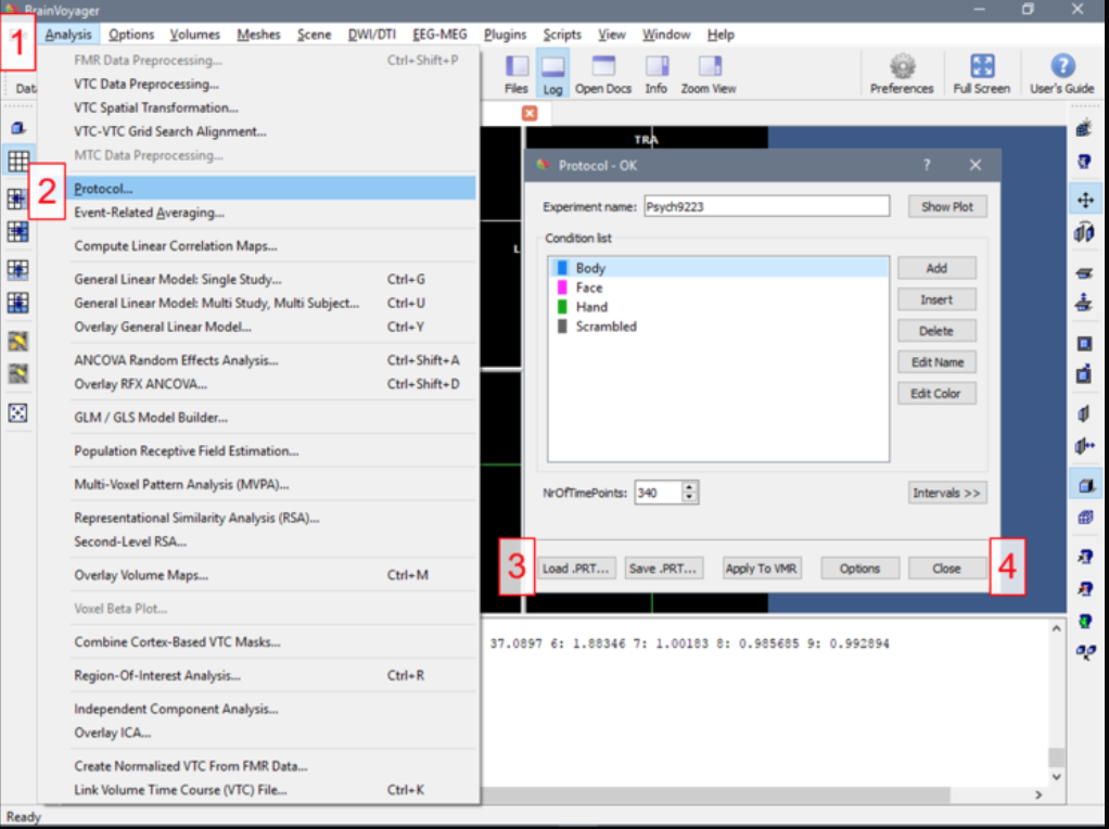
9) Close the ROI Signal Time Course window. Next, click the Analysis menu and select Protocol… Once the Protocol window opens, click the Load .PRT button and select and open Loc1.prt then click Close.
Right-click on a voxel anywhere within the boundaries of the functional data and again select Show ROI Time Course. Note that now you can see the time course superimposed on a graphical representation of the protocol.
Let's look at a specific voxel in occipital cortex. You can type coordinates in the 3D Volume Tools window (if this is closed, repeat Step 6) or you can see the coordinates for a location at the crosshairs after you have moved them by clicking in the VMR window.
Question 7: Adjust the system coords separately for the x, y and z planes and note how the crosshairs move. For example, the x coordinate changes the location in the left-right direction. What directions correspond to the y and z coordinates?

In the 3D Volume Tools window, enter the system coords for the position x=105, y=204, and z=105. Then Right-click near the crosshairs and select Show ROI Time Course. You should see the following ROI Signal Time Course appear.
Question 8: a) Does this voxel’s functional signal appear to be correlated to any of the experimental stimuli? b) Does this make sense given the voxel’s anatomical position?
Congratulations! You have successfully learned the basics of anatomical and functional MRI data files.
You can see that we could "voxel surf" -- randomly click around the expected locations of brain areas that we would expect to show activation -- but with 366,912 functional voxels, it would take an inordinately long time to look at them all! As such, we need a way to flag the voxels that show interesting patterns related to our protocol. In the next tutorial, we will learn how to use statistics, specifically the general linear model, to make maps showing us where in the brain reliable differences between conditions can be found.