Tutorial 3 - Understanding the General Linear Model (GLM)
Goals
Extend the GLM from a single predictor to a multiple predictor model
Learn how to use contrasts in statistical analyses
Understand why a correction for multiple corrections is necessary.
Understand the different options for correcting for multiple comparisons.
Accompanying Data
Background and Overview
In the previous tutorial, we gave an introduction on how to quantify the amount of activation for a given condition (i.e., beta weight) and determine whether this activation is significantly different from baseline. This tutorial will be an extension of the previous tutorial and show you how we can extract beta weights for a given number of conditions and then statistically compare them using the General Linear Model (GLM).
I. Applying the GLM to Single Voxel Time Courses
Recall in the last tutorial when we fit a visual predictor to an fMRI time course. To fit the model, we scaled the predictor and added a constant. We set these parameters in a way that minimized the residuals (i.e., explained the most data). However, our paradigms often include more than one condition. For example, the localizer run in our study contained four conditions: faces, hands, bodies, and scrambled (as well as a fixation baseline).
If we want to estimate the activation for each of these conditions, then our model will need four predictors (instead of one predictor like in the previous tutorial). Thus, each predictor will have it's own beta weight (i.e., scaling factor). The widget below shows an example of us.
Estimating Multiple Beta Weights

Widget 3-1. Fitting a 4-POI GLM to the localizer data from 3 voxels
In the following animation, adjust the sliders until you think you have optimized the model for Voxel A (i.e., minimized the squared error). You can test how well you did by clicking the Optimize GLM button, which will find the mathematically ideal solution.
Question 1:
a) What is the optimal beta weight for each predictor in Voxel A?
b) From these beta weights, what can you conclude about Voxel A's selectivity for images of faces, hands, bodies and/or scrambled images?
- Voxel A is specifically selective to hands and faces
- Voxel A is specifically selective to bodies and scrambled
- Voxel A is specifically selective to hands, faces and bodies
- Voxel A is not specifically selective to any of the 4 types of stimuli
c) Now fit the 4 predictor model to voxels E and F. What are the optimal beta weights for each predictor in voxels E and F?
d) What can you conclude about their selectivity for images of faces, hands, bodies and/or scrambled images?
- Voxel E is selective to hands and Voxel F is selective to faces and bodies
- Voxel E is selective to faces and Voxel F is selective to hands and bodies
- Voxel E is selective to faces and Voxel F is selective to hands only
- Voxel E is selective to hands and Voxel F is selective to faces only
II. Whole-brain Voxelwise GLM in BrainVoyager
In the previous section, we explained how the GLM can be used to model data (with mutliple predictors) for a single voxel. Now, we can apply this to the whole brain by fitting one GLM for every voxel in the brain.
Conducting a GLM analysis
1) Select File/Open... , open sub-10_ses-01_T1w_BRAIN_IIHC.vmr. Then attach the VTC by selecting Analysis/Link Volume Time Course (VTC) File... . In the window that opens, click Browse , and then select and open sub-10_ses-01_task-Localizer_run-01_bold_256_sinc3_2x1.0_NATIVEBOX.vtc , and then click OK .
2) Select Analysis/General Linear Model: Single Study. By single study, BrainVoyager means that we will be applying the GLM to a single run.
Click options and make sure that Exclude last condition ("Rest") is checked (the default seems to be that Exclude first condition ("Rest") is checked).
3) Click Define Preds to define the predictors in terms of the PRT file opened earlier and tick the Show All checkbox to visualize them. Notice the shape of the predictors – they are identical to the ones we used earlier for in Question 2. Now click GO to compute the GLM in all the voxels in our functional data set.

Figure 3-1. Defining predictors.

Figure 3-2. This tab on the Single Study GLM dialog allows you to exclude the baseline condition if it is the first or last condition specified.
After the GLM has been fit, you should see a statistical "heat map" . This initial map defaults to showing us statistical differences between the average of all conditions vs. the baseline . More on this later.
In order to create this heat map, BrainVoyager has computed the optimal beta weights at each voxel such that, when multiplied with the predictors, maximal variance in the BOLD signal is explained (under certain assumptions made by the model). Another, equivalent interpretation, is that BrainVoyager is computing beta weights that minimize the residuals. For each voxel, we then ask, “How well does our model of expected activation fit the observed data?” – which we can answer by computing the ratio of explained to unexplained variance.

Figure 3-3. Four predictor GLM
It is important to understand that, in our example, BrainVoyager is computing four beta weights for each voxel – one for the Face predictor, one for the Hand predictor, one for the Bodies predictor and one for the Scrambled images predictors. And for each voxel, residuals are obtained by computing the difference between the observed signal, and the modelled or predicted signal – which is simply vertically scaled by the beta weights. This is the same as you did manually in Question 2.
But we don't simply want to estimate activation levels for each condition by computing beta weights; we also want to be able to tell if activation levels differ statistically between conditions!
Comparing Activation between Conditions
Just as with statistics on other data (such as behavioral data), we can use the same types of statistics (e.g, t tests, ANOVAs) to understand brain activation differences and the choice of test depends on our experimental design (e.g., use a t test to compare two conditions; use an ANOVA to compare multiple conditions or factorial designs). Statistics provides a way to determine how reliable the differences between conditions are, taking into account how noisy our data are. For fMRI data on single participants, we can estimate how noisy our data are based on the residuals.
For example, we can use a hypothesis test to test whether activation for the Face condition (i.e., the beta weight for Faces) is significantly higher than for Hands, Bodies and Scrambled images (i.e., the beta weight for Hands, Bodies and Scrambled images). Informally, for each voxel we ask, “Was activation for faces significantly higher than activation for Hands, Bodies and Scrambled images?”
To answer this, it is insufficient to consider the beta weights alone. We also need to consider how noisy the data is, as reflected by the residuals. Intuitively, we can expect that the relationship between beta weights is more accurate when the residuals are small.
Question 2: Why can we be more confident about the relationship between beta weights when the residual is small?
We can perform these kind of hypothesis tests using contrasts . Contrasts allow you to specify the relationship between beta weights you want to test. Let's do an example where we wish to look at voxels with significantly difference activation for Faces vs Hands.
4) Select Analysis/Overlay General Linear Model... , then click the box next to Hands until it changes to [-], set Faces to [+] and the others to [].
Note: In BrainVoyager, the Face, Hand, Bodies and Scrambled predictor labels appear black while the Constant predictor label appears gray. This is because we are not usually interested in the value of the Constant predictor so it is something we can call a "predictor of no interest" and it is grayed out to make it less salient. Later, we'll see other predictors like this.
Question 3: In the lecture, we discussed contrast vectors. What is the contrast vector for the contrast you just specified?

Figure 3-5. An example contrast for Faces vs. Hands.

Figure 3-6. The voxel beta plot shows beta weights for a given voxel when you place the cursor over it. Beta weights are relative to the baseline = 0.
Click OK to apply the contrast. Use the mouse to move around in the brain and search for hotspots of activation. By doing this, you are specifying a hypothesis test to test whether the beta weight for Faces is significantly different (and greater than) the beta weight for Hands. This hypothesis test will be applied over all voxels, and the resulting t-statistic and p-value determine the colour intensity in the resulting heat map.
Question 4:
a) How can you interpret the colours in this heat map – does a voxel being coloured in orange-yellow vs. blue-green tell you anything about how much it activates to Faces vs Hands?
- Voxels colored in orange respond more to faces than hands while voxels colored in blue respond to images of hands to faces.
- Voxels colored in orange respond more to hands to faces while voxels colored in blue respond to images of faces than hands.
- Voxels colored in orange indicate strong activation to both faces AND hands while voxels in blue indicate zero activation to faces AND hands.
- Voxels colored in orange indicate strong activation to both faces OR hands while voxels in blue indicate zero activation to faces OR hands.
b) Can you find any blobs that may correspond to the fusiform face area or the hand-selective region of the lateral occipitotemporal cortex?
Corrections for Multiple Comparisons
Our whole-brain voxelwise analyses have revealed which voxels are most statistically reliable, but how will we determine which p-value cut-off (threshold) to use, especially considering that the GLM was run on ~194,000 voxels. Let's explore different options.
1) Let's start with the usual convention, p < .05.
Select Analysis/Overlay volume map . Go to the Statistics tab , select Set threshold manually and uncheck Enable Cluster threshold . Then, go to the Map Options tab. Set the p-value to .05 and click Apply .

How to turn off the cluster threshold.

How to set a map threshold to a specific p value.
Question 5: Given that a p-value threshold of .05 is the usual statistical standard, why is it suboptimal for voxelwise fMRI analyses?
2) Now apply a Bonferroni correction .
Under Map Options, ensure the p value is set to .05 but this time, check the Bonferroni checkbox and click Apply .
You can see the number of voxelwise tests performed by looking in the Statistics tab, in the False Discovery Rate section.

How to see how many voxelwise tests were performed.

Question 6: For the number of voxels tested here, what is the p-value threshold? Hint: check the p value shown under the look-up table (LUT). How is it calculated?
3) Now let's look at the effects of applying a cluster correction . Generally, cluster corrections should only be used with a p-value threshold -- here called a cluster-determining threshold -- of 0.001 or stricter. Turn off Bonferroni correction and set the p-value to 0.001 . Look at the map to remember how it looks.
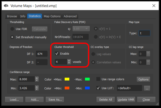
To decide on a cluster size cutoff, we ran a algorithm to compute the likelihood of getting clusters of different sizes. The output showed that the probability of finding clusters of activated voxels when no such effect is actually present(i.e., Type I errors) is below 0.05 when the cluster size is equal to 4.
In the Statistics tab, enable cluster thresholding and set the number of voxels to 4.
Question 7: You've now examined the following cases: (a) uncorrected p .05; (b) Bonferroni-corrected p .05; (c) cluster threshold correction; and (d) false-discovery-rate correction. Indicate which correction approach the following pros and cons correspond to:
- Assumes independence of voxels (no clusters)
- Good approach once you have reduced the number voxels in the analysis (e.g., region of interest)
- Handicaps small regions
- High chance of finding false positives
- In most cases a good balance of Type I and Type II error
- Has low statistical power and is more vulnerable to Type II error
- Overly conservative
- Overly liberal
- Susceptible to p-hacking
- Very conservative when there is little activation
Question 8: For each of the following situations, indicate whether you must apply correcions to minimize Type I or Type II error.
- You are looking for a robust effect.
- You are analyzing a region of interest.
- Your goal is to explore data.
- You are doing a whole-brain analysis.
- You are looking for a small effect.
- You are analyzing pilot data with very few participants.
- You are conducting a confirmatory analysis, with the aim of publishing.
Understanding bulk contrast and conjunction
In the menu, select Analysis/Overlay Maps . In the Browse tab, select Load... and load the file sub-10_ses-01_run-01_Single-Bulk-Conjunction_multimap.vmp.
The first four maps show simple contrasts . The fifth map is a conjunction of the first four. The last map is what will call a bulk contrast .
Question 9: How can you interpret the fourth contrast Hand +1 (i.e., what is Hand activation being compared to)?
You can change which map you see by clicking on the little box [+] to the right of the map to select the one you want. To see multiple maps superimposed, you can go to the Advanced tab and in the upper right Map Selection mode , select Multiple selections . Now when you return to the browse tab, you can put [+] before multiple maps to overlay them.
Let's compare these three types of maps. First, turn on the first three maps .
Question 10: Would the voxel at coordinates x = 43, y = 160, z = 101 be part of the conjunction? Why or why not? Would the voxel at coordinates x = 48, y = 160, z = 95 be part of the conjunction? Why or why not?
Now turn off the first three maps, and activate the conjuntion map ( Conjunction for Hands ). Check your answers to question 14.
Question 11:
a) Which contrast most limits the extent of activation in the conjunction? Theoretically, how could you explain this?
It can also be useful to explore the time courses of potential regions of interest to see the patterns and make sure that activation differences are not driven by noise (e.g., spikes). Find the region you think most likely to correspond to left LOTChand. Remember the data are in the radiologic convention. Move the crosshairs there, left-click to select Show ROI time course, click the green box in the lower left of the time course window to expand it, and explore the time course from the two runs.
b) In this participant's data, can you make a reasonably strong case that there is an area around the expected location of LOTChand that clearly responds more to hands than each of the other conditions? Why or why not?
Now turn off the conjunction, and turn on the bulk contrast map instead ( Hands - Body - Face - Scrambled ).
Question 12: Does this map show more or less significant activation than the conjunction? Why?
Question 13:
a) Imagine you wanted to use contrasts to find voxels that have significantly greater activation to Faces than to Hands, Bodies and Scrambled. What are two possible contrast vectors you could use to find these voxels?
- (+3 Faces) vs (-1 Hands -1 Bodies -1 Scrambled)
- +1 Face -1 Hands -1 Bodies -1 Scrambled
- (+1 Face vs -1 Hands) AND (+1 Face vs -1 Bodies) AND (+1 Face vs -1 Scrambled)
- (+3 Face vs -1 Hands) AND (+3 Face vs -1 Bodies) AND (+3 Face vs -1 Scrambled)
b) How are these two contrasts found in question 7a different from each other?
c) Which one is more liberal and which one is stricter?