Tutorial 1: fMRI Data Structures
Goals
To become familiar with anatomical and functional MRI data
To understand how functional and anatomical scans differ
To become familiar with core BrainVoyager interfaces, features, and file types
To understand how raw data from the scanner is processed and organized
Relevant Lectures
Lecture 02a: MRI and fMRI basics
Lecture 02c: Class experiment design
Lecture 02d: Introducing jargon using class experiment design
Accompanying Data and Question Sheet
Background
The data accompanying this tutorial includes data for an anatomical scan and a functional localizer scan (file prefix = sub-10_ses-01_task-Localizer_run-01_bold ) from one participant, along with several other files needed for analysis. The functional scan was one run of the localizer experiment, outlined in the Experimental Design page. In later tutorials, we will learn how to combine data across scans and participants. However, we will learn the basics with the simplest data set we can have for now — one functional run for one participant.
The strategy we use for the tutorials is like the one used in a cooking show. When you’re watching a cooking show, you don’t want to spend an hour watching someone chop vegetables, so the chef has everything done ahead of time so the viewer can watch the most important steps. Nevertheless, it is useful to understand the necessary but boring steps. The details differ from one scanner to another and from one software package to another, but the spirit of the steps is the same. Here we first review the steps in getting the data off the scanner, into common file organization structures (BIDS) and formats (NIfTI), and then into the software used here, BrainVoyager. Then we get to the good stuff, understanding the actual anatomical and functional data.
Siemens Data is stored in DICOM files
Before getting started, recall that, in most fMRI sessions, an anatomical scan is obtained in addition to any functional scans. In this tutorial, we are using scans for one participant collected at Western University’s Robarts Research Institute Centre for Functional and Metabolic Mapping using a Siemens 3-Tesla Prisma scanner. This scanner records and stores anatomical and functional images using the DICOM digital image format – a standard medical imaging format for MRI data storage and transmission.
The raw DICOMS can be made available on request; however, to reduce the size of the downloaded data, they have not been included in the data set associated with this tutorial. Nevertheless, it is useful to realize that DICOMS are the most raw form of the data from the scanner. DICOM file names end with the suffix .dcm
PRO TIP: You should always ensure your raw files are preserved in a computer backup. Do not only save the processed files. If anything goes wrong in data processing, the raw files can be used to regenerate subsequent steps. If you are scanning at CFMM, I believe the raw data get stored on their server indefinitely.
Anatomical Scans in DICOM Format
An anatomical scan is recorded as a collection of 2D images or slices of the brain. This results in a separate DICOM file for each slice. Using Horos, a free MacOS application for connecting to DICOM servers, we can easily access the DICOM files for our scan. Figure 1 is a rendering of a single DICOM file corresponding to 1 of the 176 sagittal slices of this participant’s anatomical scan. As we can see, this is in fact slice 87 (Im: 87/176), which is slightly lateral to the left-right midline of the brain. This type of scan is called a “T1-weighted” scan in which white matter appears brighter than gray matter and ventricles appear black.
Other information can also be found in the above image, such as slice thickness in mm (1 mm), 2D image size in pixels (224 x 256 pixels), the participant’s anonymized identifier (sub10), and the name of the study (Culham Psych_9223). If we were to stack the series of anatomical slices, we would have a 3D volume that covered the whole head. Given that the brain anatomy at this coarse scale does not change measurably through a session, only one anatomical volume is collected.

Figure 1-1. Single 2D anatomical image
Functional Scans in DICOM Format
Functional scans are also recorded one slice at-a-time and can also be stacked into volumes. However, the angle of the slices – chosen by the experimenters – differed from that of the anatomical slices. Here the slices were tilted off the axial (horizontal) plane. Because functional activity of the brain changes moment-to-moment, we sampled the brain not just once, but repeatedly - once per second - during each functional scan. Another way to phrase this would be to say we collected one volume per second. Note that “volume” can refer to space (specifically our 52 slices that comprise a 3D brain volume) but also to time (340 volumes/scan). Figure 2 is an example of a single functional DICOM file visualized using Horos. This is the set of quasi-axial slices that comprise one volume.
As we can see, this array contains 52 slices of functional data, and is the first volume in a sequence of 340. Together, these 52 slices provide functional data for the entire volume (in this case, the whole brain) within a 1-s period.

Figure 1-2. Single functional DICOM file
DICOM files are converted to BIDS

Figure 1-3. Example of the BIDS organization for one participant (sub-10). The folders shown contain raw BIDS data. The larger files (.gz) contain data. The smaller files (JSON and .tsv) contain header information about how the data were collected. The derivatives folder contains non-BIDS formatted data like BrainVoyager files.
The raw DICOM data from the course have been converted to a file organization and naming system called BIDS = Brain Imaging Data Structure. BIDS organizes data into folders and files with a systematic strategy and nomenclature, making it easier to share data between different labs (in the move toward open science) and across different software platforms. The BIDS file prefixes (e.g., data with the file prefix sub-10-ses-01 is from the 10th participant, who participated in their first (and only) scanning session for this experiment) have been preserved; however, to reduce the amount of data you are required to download, we have provided only the essential files and have not always preserved the BIDS file organization structure. Many BIDS filenames end in the suffix .nii.gz. nii is a suffix that indicates the file is in a format from the NIfTI = Neuroimaging Informatics Technology Initiative. Most major software packages, including BrainVoyager, can read NIfTI files. The gz suffix indicates that the file has been compressed (using gzip compression) to save space. An example is shown in Figure 3.
BIDS files are converted to volumetric 3D files in BrainVoyager
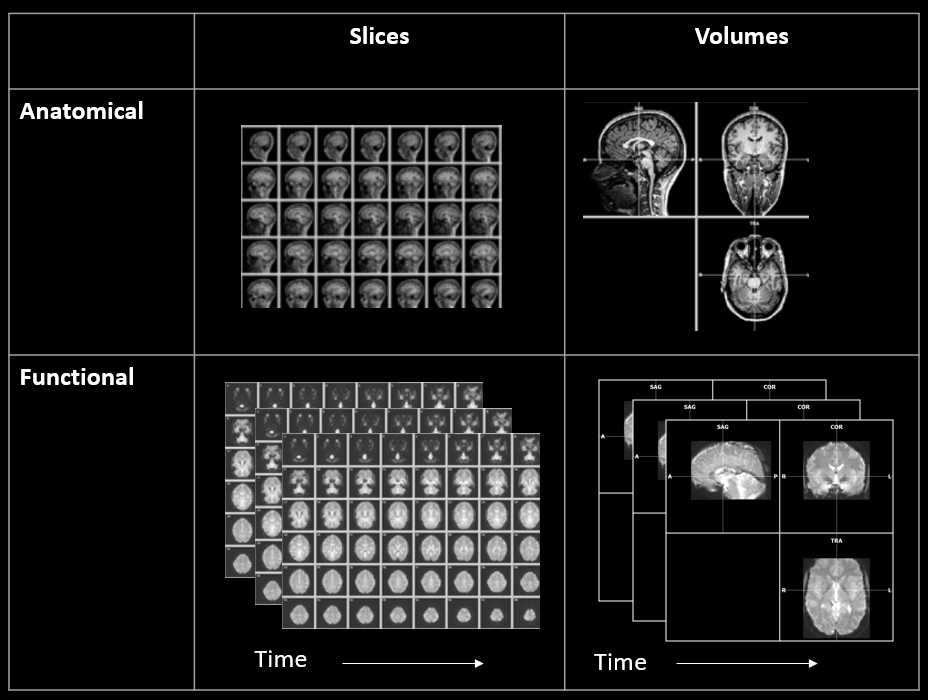
Figure 1-4. fMRI data typically include anatomical and functional scans. Data is initially stored as a matrix of 2D slices. In later processing steps, it can be converted to 3D volumes to make visualization, navigation, and analysis easier.
Each piece of software has its own file formats that may be specific to the type of data (e.g., anatomical vs. functional scans). The data were preprocessed by a Workflow Manager in the full version of BrainVoyager to convert files to software-specific formats.
In this tutorial, you will work with one anatomical scan and one functional scan. The anatomical scan files have the file prefix sub-10_ses-01_T1w, with T1w indicating that the anatomical was collected with a T1-weighted sequence. The functional scan files will have the prefix sub-10_ses-01_task-Localizer_run-01_bold to indicate that the task was the first (01) Localizer and the data was based on the BOLD = Blood Oxygenation Level-Dependent signal that fMRI measures.
As shown in Figure 4, initially both anatomical and functional data are stored as a matrix of 2D slices. However, the data are then transformed into 3D volumes shown from three orthogonal views.
One of the challenges of learning any new fMRI software, including BrainVoyager, is learning the various file types including those presented throughout the tutorial. A summary of the file types used in the tutorials is available here for quick reference.
Getting familiar with anatomical and functional MRI files
First, we will start by opening and looking at the properties of basic files in BrainVoyager.
1) Open Brainvoyager and click Accept to get started.
Viewing Anatomical Slices
2) Click File/Open... , navigate to the folder containing the tutorial data, and open the file sub-10_ses-01_T1w.amr .
You can change the number and size of the images by clicking on the left menu bar (Figure 5).
This opens an AMR (Anatomical MR) file which includes an array of 2D anatomical slices – much like the original functional DICOM files we can view in Horos. Although our analyses will use 3D anatomical files ( VMR files) instead, looking at the AMR helps you understand the data as it comes off the scanner and can sometimes be useful for troubleshooting.
Question 1: What slice plane were the anatomical images collected in?
- Sagittal
- Coronal
- Horinzontal

Figure 1-5. Contols to adjust the slice matrix dimensions
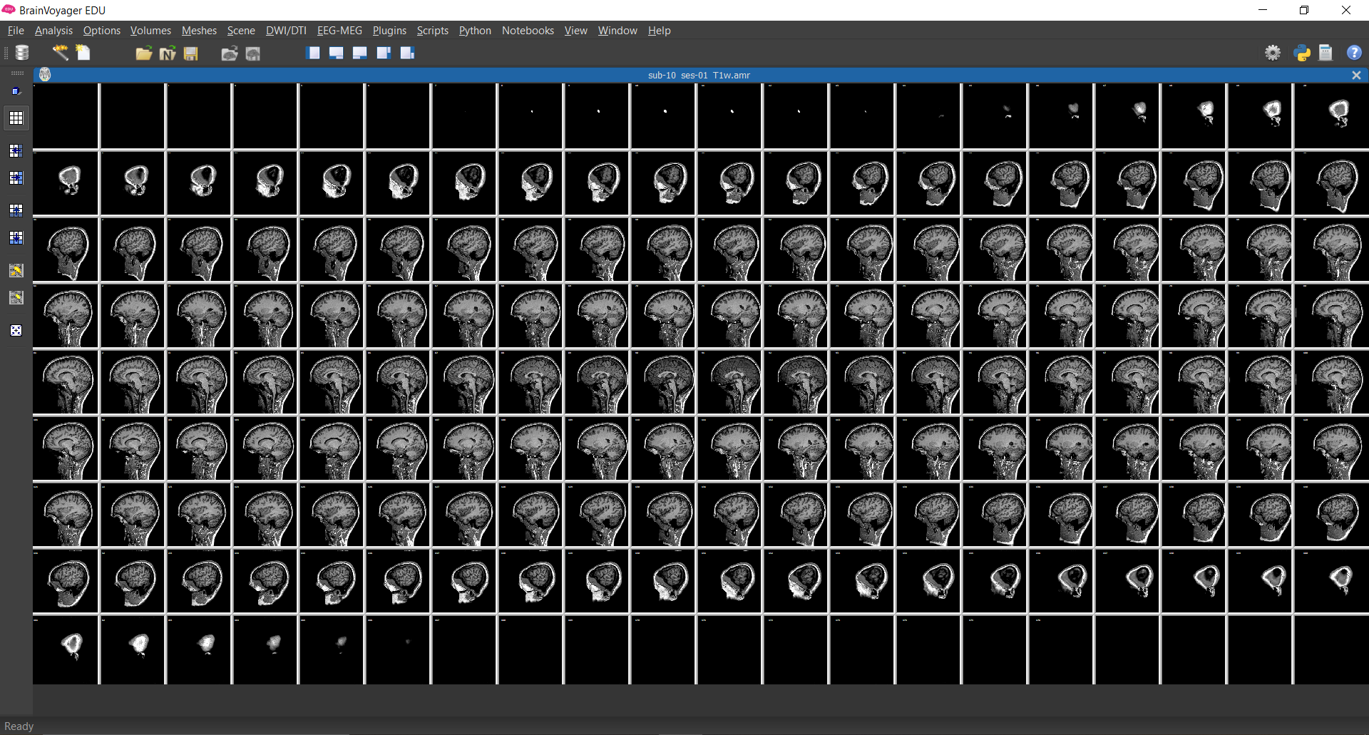
Figure 1-6. Anatomical slices shown in a 2D matrix (.amr file)
Viewing Functional Slices
3) Next click File/Open... , select sub-10_ses-01_task-Localizer_run-01_bold.fmr , and open the file.
Essentially, the FMR (Functional MR) file is a text file containing information about the functional scan, including information about the spatial and temporal resolution.

Figure 1-7. Functional slices shown in a 2D matrix (.fmr file)

Figure 1-8. The fMR properties show the key details about the spatial and temporal resolution of the scan.
Bonus question: Try opening sub-10_ses-01_task-Localizer_run-01_bold.fmr in a text editor like Notepad or TextEdit. What information is included in the file? Most of this information is also displayed in the FMR Properties window which opens automatically when opening the FMR file.
Question 2: Look closely at the FMR Properties window. (Note: If you've closed this window, you can open it again using File/Document Properties/FMR Properties)
a) What is the temporal resolution (TR)? How many time points (i.e., volumes) were sampled in this run? Given the number of volumes and the time it took to collect the volume (TR), how long in minutes and seconds did this run take?
b) The number of skipped volumes is 0. What are skipped volumes and why is it essential to fully understand whether your scanner saved the initial dummy scans or not?
c) What was the original or “raw” spatial resolution of the functional scan? Are the voxels isotropic or nonisotropic?
Opening an FMR (text) file also automatically reads in the associated STC or Slice Time Course (data) file (in this case Sub-10_ses-01_task-Localizer_run-01_bold.stc ). Keep in mind that a functional scan involves multiple time points and therefore functional data is comprised of mulitple slice arrays (volumes) over time. Although, opening an FMR file will show you the array of functional slices for the first time point only, we can visualize the 4th dimension (time) by watching the arrays as a movie.
4) Close the FMR Properties window , then select Options/Time Course Movie . Then click Preload All , wait roughly 5 seconds, and click > to visualize each the functional data over time.
Click the First<->Last button to toogle between the first image that was acquired and the last one.

Figure 1-9. Time course movies allow you to visualize functional volumes over time to check for head motion and other artifacts.

Seeing small changes might be difficult when looking at all the slices at once. You can also view the movie for single slices. Using buttons on the left toolbar (with the blue arrows), zoom in until you only have one slice (square) on your screen . Once you've zoomed into a single slice, you can move between slices using the left and right arrow keys . Now try viewing the movie for slices at the bottom, middle, and top of the brain.
This is a simple, important step for performing basic quality assurance of your functional data.
Question 3:
a) What might you determine by viewing the Time Course Movie? Select all that apply.
- You can determine whether the participant moved during a run.
- You can determine in which areas of the brain were active during the scan.
- You can determine whether there are susceptibility artefacts.
- You can determine whether there were any scanner malfunctions.
- You can determine what the participant was thinking about.
b) Do you think this is good quality data? Why or why not?
Viewing Anatomical Volumes
5) Click Open , navigate to the folder containing the tutorial data, select sub-10_ses-01_T1w.vmr , and open the file.

Figure 1-10. Anatomical data shown in a 3D volumetric view (.vmr file)
This VMR provides a 3D view of the anatomical scan generated by "stacking" the 2D slices in a third dimension. The VMR shows three orthogonal planes (sagittal, coronal, and horizontal) centred on a single point (the white crosshairs). Try moving one of the crosshairs to change the view! Note that the views in the other two slice planes change accordingly. It is much easier to get your bearings in a 3D view (the VMR) than the 2D slice arrays (the AMR), which is why we'll be using only the VMRs from this point forward.
Click File/Document Properties/VMR properties .
Similar to the FMR Properties window (functional slices), the VMR Properties window can give you important information about your data.
Question 4:
a) In what type of view are the images present in? To what side of the brain does the left side of the image correspond to in the coronal view? Fill in the blanks.
The images are presented in the __ view, which means that the __ side of the image in the coronal view corresponds to the __ side of the brain.
b) What is the spatial resolution of the image? Select all that apply.
- 1 mm isotropic
- 1 mm3
- 1 x 1 x 1 mm
- (1 mm)3
- 1 mm x 1 mm x 1 mm
c) How many time points does this file have?
- 1 time point
- 340 time points
- 680 time points
- None of the above
Now that we have the anatomical scan in 3D ( VMR ), we also want to look at the functional scan in 3D (VTC ).

Figure 1-11. Showing VMR propeties.
Viewing Functional Volumes
6) Click Analysis/Link Volume Time Course (VTC) File... and select the file sub-10_ses-01_task-Localizer_run-01_bold_256_trilin_2x1.0_NATIVEBOX.vtc .

Figure 1-12. To use or visualize functional data, after opening a .vmr file, link it to a .vtc file.
The VTC file provides a 3D view of the functional scan, and, similar to the VMR file, is generated by "stacking" the 2D functional slices in a third dimension. In addition to stacking, the VTC file undergoes two other types of transformation. The functional data is first resampled to a resolution of either 1, 2 or 3 mm isotropic, and then it is aligned to the anatomical data. This will allow us to use the participant’s brain anatomy to guide preliminary functional analysis.
Seeing as we wish to focus more specifically on data analysis, steps invovled in generating the VTC file will be done for you. For now, step 6) allows you to link a VTC that we have generated for you to the anatomical data (i.e., the VMR file).
Open the VTC file properties by clicking File/Document Properties/VTC properties .
Question 5:
a) What is the spatial resolution of the functional image? Select all the correct ways of reporting the spatial resolution of this functional image.
- 8 mm
- (2 mm)3
- 2 x 2 x 2 mm
- 2 mm isotropic
- In-plane resolution of 2 mm with a slice thickness of 2 mm
b) Compare the spatial resolution from the DICOM file (Figure 2 at the very beginning of this tutorial) with the spatial resolution of the VTC file. In one sentence, why are they different?
c) Now, compare the spatial resolution of the VMR(anatomical volume) and VTC (functional volume). How many anatomical voxels would fit in one functional voxel?
- 1 voxel
- 2.5 voxels
- 2 voxels
- 4 voxels
- 8 voxels
- 15.625 voxels
Differences between functional and anatomical volumes
Before comparing anatomical and functional images, we will introduce you to a useful tool called 3D Volume Tools.
7) Click on the blue box at the top of the menu bar on the left side of your screen (hereafter affectionately called "blue box mode"). The 3D Volume Tools window will appear in minimized dialog box, which you can change to the full dialog box by clicking Full Dialog.

Figure 1-13. You can visualize and control many features of 3D volumetric data by opening “blue box mode”.

Figure 1-14. The reduced window for blue box mode shows only the 3D coordinates. To expand the view, click the “Full Dialog >” button.
The first thing you will notice is the x, y, z coorinates in the 3D Coords tab. When moving the cursor, you will notice that the coordinates displayed in the window change according to the cursor's position.
Question 6: Which axis (x, y, z) correspond to each direction: front-back, up-down and left-right, anterior-posterior, dorsal-ventral?

Figure 1-15. The full window for blue box mode gives many more options.
8) Next, go to the Spatial Transf tab, and look at the section called Show a volume of attached VTC data.
As mentioned above, once you've attached the functional data to the anatomical data, you can go back and forth between the two types of images. If you click on Show VTC , a functional volume will be displayed instead of the anatomical volume(Note: there is a quicker way of doing this in the next paragraph). Furthermore, remember that functional data has a fourth dimension, namely time. In order view functional volumes at different time points, simply change the number on the right of the Show VTC button to the desired volume.
In the same section, there is a box labeled Trilinear interpol. Try checking and unchecking this box and using the Show VTC button after each change. (Hint: Use the short key ctrl+t to toggle from a 3-slice to single slice view.) Notice that checking the Trilinear interpolation box makes the image look much smooth, whereas leaving it unchecked makes the image look more pixallated. We will keep the Trilinear interpol. box unchecked in future steps and tutorials to help you keep in mind that the actual data is pixellated (voxelated?).
Figure 1-16. To visualize one volume of the 3D functional data, click “Show VTC Vol” for the volume number you want to see.

Figure 1-17. Sagittal slice without trilinear interpolation

Figure 1-18. Sagittal slice with trilinear interpolation
Finally, it's important to remember that, although they overlap a great deal, anatomical and functional images are different. This can be easily seen when toggling between the anatomical and functional images. To toggle between different types of views, press F8 . These differences become even clearer once we strip the images of useless voxels outside of the brain.
9) Click Volumes/Extract Brain from Head MRI Volume .
Question 7: Toggle again between the VTC and VMR. Name at least two out of the three major differences between the functional and anatomical images.
Question 8: On the VTC view, set the coordinates to x = 36, y = 136, z = 126 using the blue box mode and inspect the functional image. Now set the coordinates to x = 97, y = 63, z = 120 and inspect the functional image.
Indicate for each of the following statements whether they are true or false. If a statement is false, provide a short explanation as to why it is false.
- This participant must be warned that they have severe brain atrophy.
- The dark spot at coordinates x = 97, y = 63, z = 120 are caused by liquid in the sinuses.
- The dark spots at both coordinates are susceptibility artefacts.
- The dark spot in the image at coordinates x = 36, y = 136, z = 126 are caused by air in the ear canal.
Viewing time courses
The last thing we will learn to do in this tutorial is how to look at functional data time courses. Recall that functional MRI data is not just 3D but 4D, with the 4th dimension being time. We can examine the time courses of single voxels or larger regions. It can also be valuable to inspect time courses to understand what the raw data looks like and what types of artifacts might be present.
10) To examine these time series, simply use the mouse to right click over any area of the brain and select Show ROI Time Course (ROI stand for Region of Interest).

Figure 1-19. Viewing time courses.

The interpretation of the time courses is more meaningful if we know how they relate to the events in our expereiment. Close the ROI Signal Time Course window.
11) Click Analysis/Protocol… Once the Protocol window opens, click the Load .PRT ... button and select and open sub-10_ses-01_Localizer_run-1.prt then click Close .

Figure 1-20. A protocol file shows the order of conditions for a given scan.

Now you can right-click on a voxel anywhere within the boundaries of the functional data and again select Show ROI Time Course . Note that now you can see the time course superimposed on a graphical representation of the protocol. You can choose to show or hide the condition labels by right clicking on the time course and selecting Show/Hide conditions.

Figure 1-21. A time course superimposed on a protocol.
Question 9: In the 3D Volume Tools window, enter the system coords for the position x=109, y=204, and z=105. Then Right-click near the crosshairs and select Show ROI Time Course. You should see a ROI Signal Time Course that appears similar to the one shown.
a) Does this voxel’s functional signal appear to be correlated to any of the experimental stimuli?
b) Does this make sense given the voxel’s anatomical position?
You can see that we could "voxel surf" -- randomly click around the expected locations of brain areas that we would expect to show activation -- but with 366,912 functional voxels, it would take an inordinately long time to look at them all! As such, we need a way to flag the voxels that show interesting patterns related to our protocol...
Viewing regions/voxels of interest (VOI/ROI)
Finally, we will how to view specific voxels/regions, a skill that will be useful for later analyses.
1) Select Analysis/Region-Of-Interest Analysis... Doing this will open the Region-Of-Interest Analysis window. Click Load... and open the file Voxels of Interest.voi . You will have noticed that there are 6 voxels (A to F) of interest in this file.
2) Expand the window by clinking on the > icon. Now we will link the .vtc to the .voi . Click Add... and open the sub-10_ses-01_task-Localizer_run-01_bold_256_trilin_2x1.0_NATIVEBOX.vtc .
Now you can click on any voxel in the VOI list and click Show Time course .

Figure 1-22. The Region-/Volume-of-Interest dialogue allows you to view time courses for a specific region (or here, voxel).
Conclusion
Congratulations! You have successfully learned the basics of anatomical and functional MRI data files.
In this tutorial, we learned about the 4 basic files formats used in fMRI analyses and, more importantly, their respective data structures. Important elements to remember for future tutorials include:
How to open an anatomical volume file (.vmr)
How to link the function volume file (.vtc) to the anatomical volume file (.vmr)
How to access properties for different types of files and understand what these properties are
How to use the “blue box mode”
How to visualize time courses
In the next tutorial, we will learn how to use statistics, specifically the general linear model, to make maps showing us where in the brain reliable differences between conditions can be found.