Tutorial 8 - Group GLM and ROI Analysis
Goals
To explore anatomical and functional variability between subjects
To understand group alignment into stereotaxic (MNI) space
To learn how to set up a group analysis in the GLM
To understand the difference between FFX and RFX analysis
To explore and understand various approaches to voxelwise and ROI-based analysis for group data
To appreciate the difference between independent and non-independent definitions of regions
Relevant Lecture
Lecture 07a: Standardization
Lecture 07b: Group GLM
Lecture 07c: Group GLM example
Lecture 07d: Regions of Interest
Accompanying Data
BV EDU Access File
If any files do not work, you may have to update your BV EDU access file and add the eduexdat.bin file from the data folder
Background
There are two issues we need to solve to do group analyses.
- We must get the brains into a common space . This could be stereotaxic space (MNI or Talairach space) or it could be cortical (surface) space. One problem with this is that even when participants are aligned in a common space, there can still be variability in the locations of functional areas across participants. This problem is worse for stereotaxic space than cortex-based alignment in surface space.
We must find a way to combine data statistically across participants. There are two ways to do this:
A. Voxelwise Whole-Brain Analysis . Combine all the participants in a common space and do a contrast across every voxel to find those with a significant effect. Here, we have to worry about the problem of multiple comparisons and use a method to control for them.
B. Region-of-Interest Analysis in which we investigate the statistics for known regions. Here, we are only doing one statistical test per region, so if we do any correction for multiple comparisons, it only need be over the number of regions tested (though realistically, most researchers don't correct for this).
Regardless of whether we are doing a voxelwise whole-brain analysis or a region-of-interest analysis, analysis of group data is considered a second-level analysis. Let's consider what this means.
First-level analysis = fit a GLM to each participant's data to estimate individual activation levels -- i.e., beta weights -- for each condition of interest.
Second-level analysis = once you have beta weights for conditions, you can now do standard statistics on those beta weights. These can include t tests (to compare two conditions) or ANOVAs (to evaluate main effects and interactions in factorial designs). These stats are the ones you've grown to know and love (or more likely hate) from your undergrad stats classes. The only difference is that the values being tested are estimates of activation levels -- i.e., beta weights -- rather than say behavioral measurements.
Recall from Lecture 2 and Tutorial 2 that statistics require a comparison of measurements (or differences between measurements) to some source of variability. In the single-participant analyses we have conducted so far, the noise term was from variability over time , i.e., residuals (df = volumes - 1 - #model_predictors). Because we only had one participant, that was the only option. With a group of participants , however, we can base the noise term on the variability over participants .
Typically in research, we want to be confident that our results are NOT due to sampling error. Here, we randomly sampled 18 participants from a population (mostly Western University grad students, TBH). However, we want to draw conclusions about the population, not the sample. That is, we want to be confident that if we were to draw any sample from that population, we would reach the same conclusions. We do not want to just draw conclusions about the 18 participants we happened to sample. Note that if the population from which we sampled (grad students) is not representative of the general population, nothing we do statistically can fix this. We assume this is less of a concern for a perceptual experiment like ours than other experiments where indidivual factors (e.g., age, education) may be more important.
If we have a reasonable number of participants, we can estimate how variable their results are and thus estimate how likely we would be to find a particular result even if we drew a different sample. This is called a random-effects analysis (RFX) . It means we are treating participant sampling as a random factor. Geek note: In some software, this approach is termed a mixed-effects analysis. Note that most of the stats you will have encountered in undergrad stats classes will be RFX analyses because you are considering effects in light of individual variability, allowing to generalize your results to the population.
RFX analyses are the most common approach to group data in fMRI; however, there is another option: fixed-effects analyses (FFX) . FFX analyses do not take into account interesubject variability and thus only allow you to draw conclusions about the specific sample you tested. FFX analyses are rarely used in fMRI but may warrant consideration in rare cases (e.g., examining pilot data where the sample size is too small to employ RFX). Because FFX analyses model each participant separately, they can provide a convenient way to investigate contrasts in individual participants for quality assurance purposes (which is easier than making one GLM, map and contrast per participant).
This tutorial will first have you explore the first issue, normalizing data into a common space, and then the second issue, combining data statistically across participants.
Comparison of Two Participants in MNI Space
First, let's compare the overlap between the anatomicals of two participants (P02 an P03) whose brains have both been transformed into MNI space.
Open sub-03_ses-01_T1w_IIHC_MNI.vmr
From the File menu , select Load Secondary VMR… , and open sub-15_ses-01_T1w_IIHC_MNI.vmr
Use a keyboard shortcut F8 on PC or Function-F8 on Mac to toggle between the two brains. You can move the crosshairs around to see different slices. Look for the hand knob of sensorimotor cortex (S1/M1). It should look like an upside-down omega.
Question 1: How well do the two brains align? Pay attention to the overall shape of the brain and to sulcal landmarks. What are the consequences of intersubject misalignments?
Comparison of MNI Template and Group-Averaged Anatomical
Next, let's look at the MNI template and an the anatomical scan averaged across participants.
From the File menu, open the MNI VMR file to see the MNI152 template.
Question 2: What features (e.g., sulci) are clear in the MNI template? Which are blurry? What does this tell you about the intersubject consistency of these features?
Then, select File/Load Secondary VMR and load sub-03_ses-01_T1w_IIHC_MNI.vmr .
You can again use F8 on PC or Function-F8 on Mac to compare between them.
Figure 1 shows a screenshot of the average T1 anatomical from 18 participants in MNI space, centred around the hand knob. CORRECTION FOR FUTURE: MAKE THIS FILE COMPATIBLE WITH BV EDU.
Question 3: In figures, researchers can render group functional activation on a template brain, an average anatomical brain, or an individual anatomical brain? What are the pros and cons of each choice?

Figure 8-1. Screenshot of the average T1 anatomical from 18 participants with crosshairs near the hand knob.
Contrasting FFX and RFX Models
In Tutorial 5, we saw how we could combine mulitple runs from a single participant. Now we will see how we can combine multiple runs from mulitple participants. We tested 18 participants. Of those, 17 participants did two runs of the localizer and one participant (s16) only did one run of the localizer due to experimenter error. As such, we have 35 localizer runs (18 x 2 - 1). For each of the 35 runs we need a SDM (Single Design Matrix) file, which contains the time courses for each of the predictors (POIs and motion PONIs) for GLM analysis. We made a multi-subject design matrix, MDM file. This files specifies the runs that we included and the predictors (single design matrix, sdm) for each participant. It also specifies the choices we made about the analysis.
Fixed Effects with Separate Subject Predictors (FFX)
We can improve the model by creating separate predictors for each participant. That is, instead of using 4 predictors (Body, Face, Hand, Scrambled) to fit the data, we could use 4 (Body, Face, Hand, Scrambled) x 18 subjects = 72 predictors/betas. This means, for example, that the beta weight for Face could be different for each subject. This is a FFX GLM WITH Separate Subject predictors (abbreviated SPSB in file names) [Side note: We could even have separate predictors for each of the two runs (or "studies" in BrainVoyager speak) for each subject -- this is what the "Separate study predictors" tick box does. However, since participants are usually fairly consistent in the magnitude of activation they show between runs, this typically is NOT done unless someone is interested in how activation changes throughout the session, e.g., as in learning studies].

Figure 8-3. This is the same multi-subject design matrix as in Figure 2 but now with separate subject predictors.
Random Effects Analysis (RFX)
By ticking the "RFX GLM" button, we change how the statistics are calculated.

Figure 8-4. This is the same multi-subject design matrix as in Figure 2 but now with RFX GLM enabled.
Question 4: In BrainVoyager, as soon as you click "RFX GLM", it turns on Separate subject predictors. Why?
Question 5: For consistency, we have turned on "Correct serial corr." in both models. Of these two situations, when is it imperative to do this correction and when is it not?
BrainVoyager has a function called ROI-GLM (Note: In BrainVoyager, Region of Interest = Volume of Interest). This allows you to take the average time course from a ROI/VOI and run a GLM on it. This can be a useful way to understand the data.
We have run three ROI GLMs for the Left LOTChand, as defined by a 7-mm-radius sphere centred on the hotspot of activation for a search of "hands" in neurosynth.org.
Open each ROI-GLM output in a separate browser window by clicking the hyperlinks below.
- FFX-SPSB Fixed Effects GLM (with Separate Subjects Predictors)
- RFX Random Effects GLM
The first section of each output file shows the results of the model without a correction for serial correlations. The next part shows the results of a model with a correction for AR(1) and AR(2). For each model, we have performed a contrast of Faces vs. Hands.
Focus your attention on the ANOVA table at the beginning for FFX. The tables show the number of degrees of freedom. For the RFX model, the degrees of freedom are indicated in the section labelled "Random effects analysis of contrasts".
Question 6: For each model, what determines the degrees of freedom (don't worry about exact df)? Which statistical model is based temporal variability and which is based on intersubject variability?
Consider the t values for the contrast of Faces vs. Hands in each approache. For consistency, consider these values after the correction for serial correlations in all cases.
Question 7: How do the t values compare? Why are they different?
RFX Contrasts Using Microsoft Excel
The beta weight outputs from the RFX GLM have been imported into Microsoft Excel and simple conventional statistics have been applied. Download the Excel file.
Question 8: What do the values entered into the spreadsheet reflect? Were the values generated from a first- or second-level analysis?
Question 9: In addition to doing a contrast in BrainVoyager, the Excel spreadsheet provides you with three additional ways you could test for statistical significance for the contrast of Faces vs. Hands. a) What are these three ways? b) How well do the t values and/or significance levels of these three approaches compare? c) Are theses tests first- or second-level analyses?
Question 10: A behavioral researcher does a conventional paired-samples t test on within-subjects reaction times for two cognitive tasks. Is she doing a random effects or a fixed effects analysis? How is a t test done on fMRI different from a t test done on behavioral measures?
Voxelwise FFX and RFX Models
We have generated voxelwise GLMs for each of the three approaches. Here are the screenshots from each of the three model outputs.

Figure 8-5. FFX GLM Output (without Separate Subject Predictors)

Figure 8-6. FFX GLM Output (with Separate Subject Predictors, SPSB)
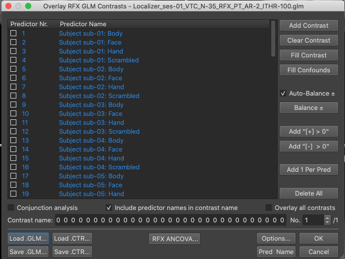
Figure 8-7. RFX GLM Output
Question 11: If the output of FFX and RFX look identical, how are their statistics actually different?
Question 12:
a) In BrainVoyager, for FFX SPSB models, you can examine contrasts for single participants, e.g., +Subject sub01:Face -Subject sub01:Hand. Why would you ever want to do this?
b) For RFX models, if you click the same settings in an RFX GLM, it will fill the Face condition with + and the Hand condition with - for every participant. Why?
Now let's compare the maps from the Faces > Hands contrast in the three models.
Close all the windows in BrainVoyager.
Select File/Open MNI VMR.
Select Analysis/Overlay Volume Maps… and load Face_Greater_Hand.vmp

Figure 8-7. We have created maps for the contrast of Faces > Hands for each of the three model types.
Use the dialog box in Figure 8-7 to alternate between the three maps by placing a + sign to the left of the map you want to view.
Question 13: Which map has the least activation at the same threshold. Why?
Question 14: These data were spatially smoothed with an 8-mm Gaussian kernel. Why is spatial smoothing important for group analyses?
Individual ROIs and the Problem of Intersubject Variability
With the MNI VMR open, select Analysis/Overlay Volume Maps and load Face_Greater_Hand_Individual.vmp .
If you want to see the expected location of LOTChand or FFA, you can examine the foci from Neurosynth.
Select Analysis/Region-of-Interest Analysis and load neurosynth_radius_7mm.voi . Select the region you want and click Show VOI . This will centre the crosshairs at the expected location. If you want to remove the coloring, click Hide VOI .
In the Overlay Maps dialog box, toggle between individual maps for the Faces > Hands contrast. Each individual's map has been thresholded using FDR correction.
Another way to examine intersubject consistency is to make a map of how many participants have overlapping activation (after thresholding) for each voxel.
With the MNI VMR open, select Analysis/Overlay Volume Maps , and load Probability_Maps.vmp . This map shows the percentage of participants that had overlapping activation at any point.
Try adjusting the percentages in the Threshold panel of the Overlap maps dialog. Note that percentages here are in whole numbers not decimals (e.g., 20% = 20 not 0.2).
Question 15: How well do participants' data overlap at the expected locations of LOTChand and FFA?
Voxelwise vs Region-of-Interest Approaches
For our main course experiment, we wanted to know whether brain areas selective for faces or hands were tuned to direction of the gaze or the index finger. For example, one hypothesis might be that LOTChand would show more activation for hands directed forward than sideways. Let's consider different ways we could test this specific hypothesis.
Question 16: How could we answer this question with a voxelwise analysis? What are the major pros and cons of this approach?
Question 17: If we localized LOTChand from the main experiment data using a contrast of Hands > Faces and then tested differences between all 6 conditions, which of the following would be independent and which would be non-independent?
- Main effect of stimulus
- Main effect of orientation
- Interaction between stimulus and orientation
Question 18: How could the localizer data be used to identify LOTChand. Suggest two ways and the pros and cons of each.
Question 19: Suggest one way we could we do a region-of-interest approach for LOTChand without needing to collect localizer data.