Tutorial 7 - Event-Related Data Analyses and Deconvolution
Goals
Understand why event-related designs can be useful
Understand the concepts of detection and estimation
Understand event-related averaging
Understand how event-related data can be analyzed with either a classic GLM or a deconvolution GLM
Relevant Lecture
Lecture 05a: Event-related averages
Lecture 05b: The imperfections of the hemodynamic response function
Lecture 05c: The problem of event history
Lecture 05d: Design types (Block, Event-related, Mixed)
Lecture 05e: Deconvolution of event responses
Accompanying Data
Background
Why Use Event-Related Designs?
Block designs have many advantages. They have the best statistical power of all designs and they are quite resilient to differences between the actual and modelled hemodynamic response functions (HRFs). As such, block designs are the default approach for fMRI. Block designs are excellent for Detection = finding blobs of activation showing differences between conditions. However, because block designs just measure the aggregate response to a series of trials, we cannot determine the detailed time course of the response to a single trial.
Compared to block designs, event-related designs are better for Estimation = extracting the time course for a type of event (trial).
Event-related designs are preferable for some types of experiments:
- Experiments where estimation of the time course is important. Estimation is important when you want to explore the time course of activation for different trials or different phases of a trial (e.g., stimulus-delay-response) without too much cross-contamination.
- Experiments with unpredictable or uncontrollable trial types. As one example, in a memory study one may wish to compare responses to familiar vs. unfamiliar items without having familiarity blocked (and thus entirely predictable by the participant). As another example, one may want to compare correct vs. incorrect trials when performance can not be controlled.
- Experiments with a large number of conditions. Because block designs typically have relatively few blocks (compared to the number of trials in an event-related deisgn), they can make it difficult to match order history across conditions.
- Experiments in which data may be contaminated by motion artifacts that are correlated with the paradigm. For example, in studies of speech or actions, there may be artifacts related to bodily motion (even if the head itself stays still). In such cases, the hemodynamic lag is actually beneficial beccause artifacts happen immediately while activation is seen with the expected lag. As such, the artifacts can be modelled with PONIs to get a better estimate of the BOLD response.
One approach is to use Slow Event-Related Designs, with long rest periods (intertrial intervals, ITIs) between trials (e.g., 12-30 s ITIs). The benefit of slow ER designs is that they provide good Estimation of trial time courses. The cost is that they yield poor Detection of activation differences because there are so few events in a run or a session.
Ideally we want both good Detection and good Estimation. Good News! A "Goldilocks" design that gives us the best of both worlds is available: Jittered Rapid Event-Related Designs
What is a Jittered Rapid Event-Related Design?
- Event-related = examines responses to single trials
- Rapid = trials are spaced close together
- Jittered = trial spacing is not entirely regular
We used such a design for our experimental runs. Recall that we had six trial types. These trial types were placed in pseudo-random order (actually counterbalanced for n-1 trial history) with a default stimulus onset asynchrony (SOA = the time between the start of one trial and the next) of 4 s, with occasional gaps of 8 s. In the actual experiment, we had 6 (or occasionally 7) runs per participant, with each run having a different order of trials.
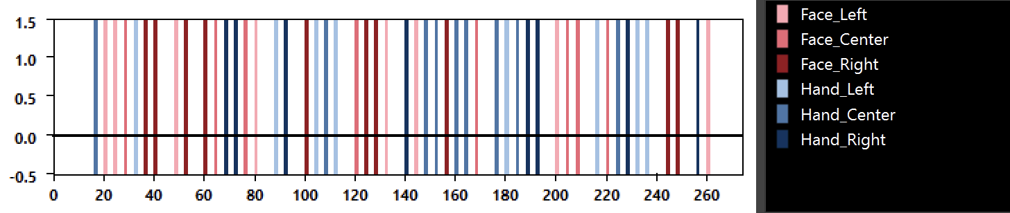
Figure 7-1. Protocol for one order of the main experiment, showing a jittered rapid event-related design in which trials were spaced every 4 or 8 s in an optimized order that balanced the n-1 trial history.
How Are Jittered Rapid Event-Related Designs Analyzed?
- We can analyze event-related data using the same Classic GLM Approach that we used for block-design data. As then, we make predictor functions that we generate from square-wave functions convolved with the default HRF, estimate the beta weights, and do statistical contrasts between conditions.
- We can also analyze event-related data using a Deconvolution GLM Approach which enables a more fine-grained analyses of the the BOLD signal. Although this approach also uses predictors, beta weights, and contrasts, the key differences are that (a) instead of using one predictor per condition with an assumed Hemodynamic Response Function (HRF), we use a series of "stick predictors" and thus do not have to assume any specific HRF.
Here you will see examples of both approaches to analyzing Event-Related data using our experimental data with 7 runs from 1 Subject (sub-15). We will first explore the Classic GLM Approach and then the Deconvolution GLM Approach.
1. CLASSIC GLM APPROACH
Participant 15 completed 7 runs of the Main Experiment, each with a different order.
The predictors for each run were created in the usual way. For each condition, we made a box car (square-wave) predictor and convolved it with the default (two-gamma) hemodynamic response function.
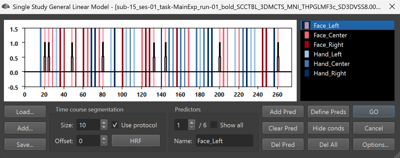
Figure 7-2. The box car predictor for the Face_Left condition.
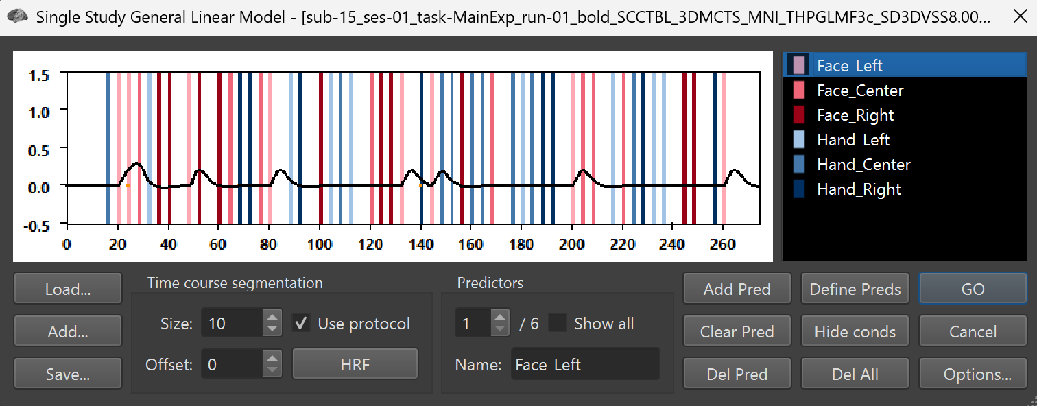
Figure 7-3. The convolved predictor for the Face_Left condition.
Question 1: In the convolved predictor for Face_Left condition (palest pink condition), why is the maximum y value less than 1 (when the box car maximum = 1)? Why is the first "bump" higher than the later bumps?
In addition to the set of predictors of interest (6 POIs), we also created predictors of no interest(6 motion PONIs) for each of the runs.
1) Select File/Open... and open file sub-15_ses-01_T1w_IIHC_MNI.vmr. Then, click Analysis/Link Volume Time Course (VTC) File... and select the file sub-15_ses-01_task-MainExp_run-01_bold_SCCTBL_3DMCTS_MNI_THPGLMF3c_SD3DVSS8.00mm.vtc
2) Select Analysis/General Linear Model: Single Study... and load the file sub-15_ses-01_MainExp_run-1_MotionPONI.sdm By checking the boxes Use Protocol and Show all, you will see all 6 POI and 6 PONIs. Do not click GO as we have already done this step for you.
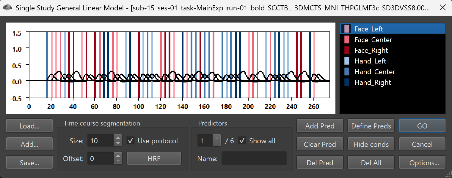
Figure 7-4. All 6 predictors of interest superimposed.
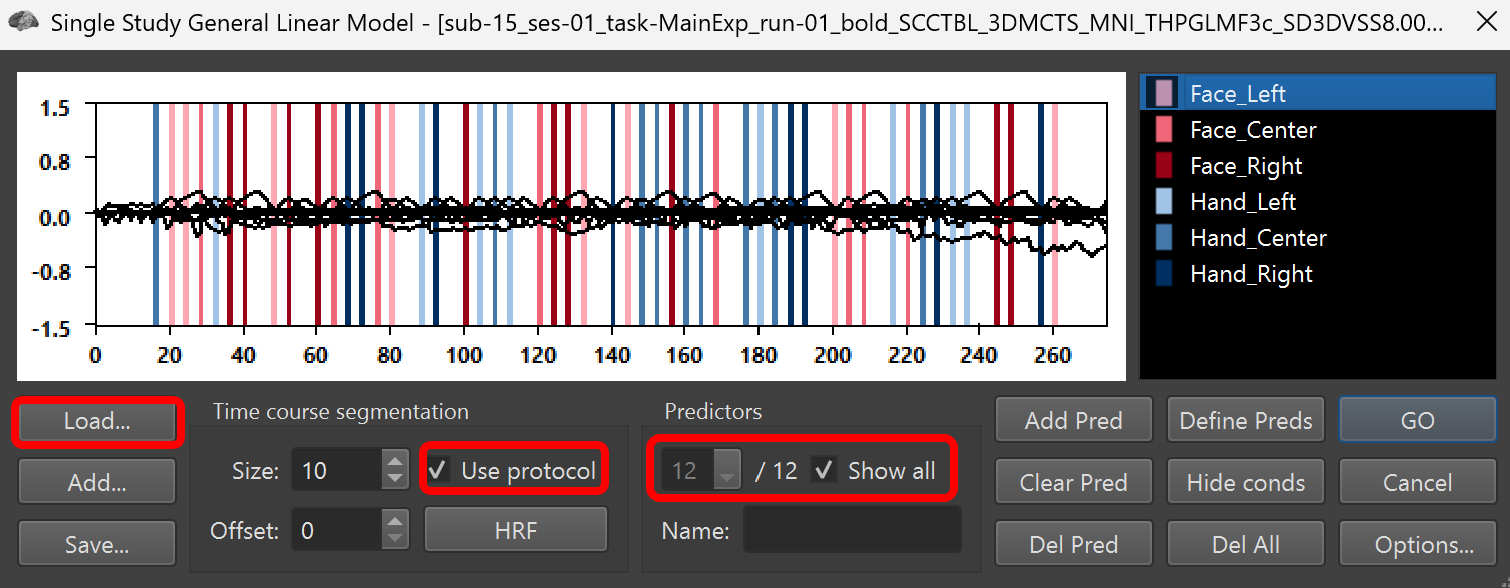
Figure 7-5. All 6 predictors of interest + 6 predictors of no interest (motion parameters) superimposed.
As usual, once we generated a single-study design matrix for each run, we entered them into a multi-study (here multi-run) design matrix. For this experiment, the contents look like this.
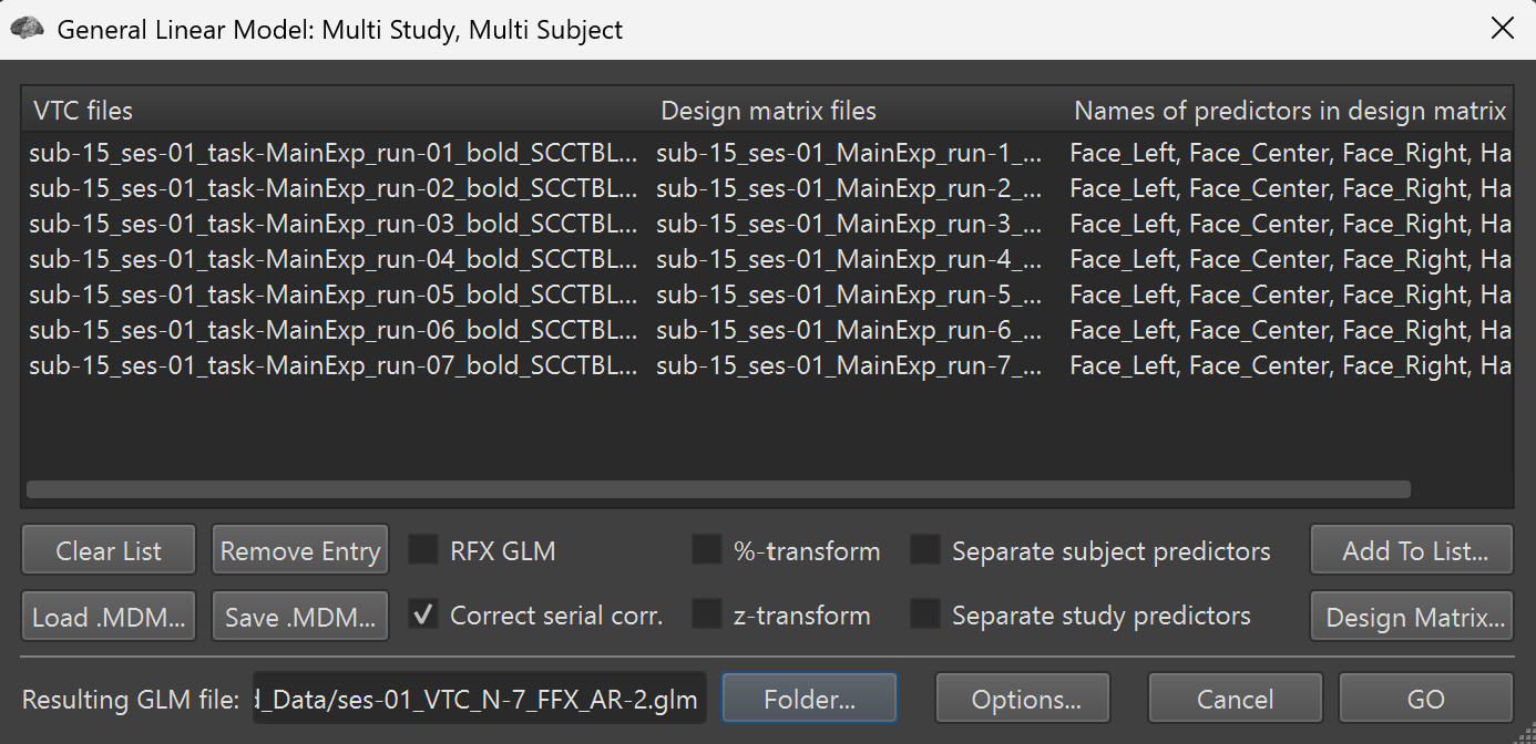
Figure 7-6. The multi-study design matrix for the 7 runs of the experiment for Subject 15.
We have already computed the GLM from this MDM.
3) Select Analysis/Overlay General Linear Model and load the file sub-15_ses-01_VTC_N-7_FFX_PT_AR-2_ITHR-100_Standard.glm . This model has estimated the beta weights for each condition across the data from all 7 runs. Because we only have data from one participant and thus our source of variance must be the residuals, the GLM employed a correction for serial correlations (as indicated by AR-2 in the filename).
When looking at the GLM, note that we have many predictors of no interest (7 for each run = 6 motion PONIs + 1 constant).
4) Assign the contrast based on the values below to compare Faces > Hands (each collapsed across the three orientations):
+Face_Left +Face_Centre +Face_Right -HandLeft -HandCentre -HandRight
Click GO.
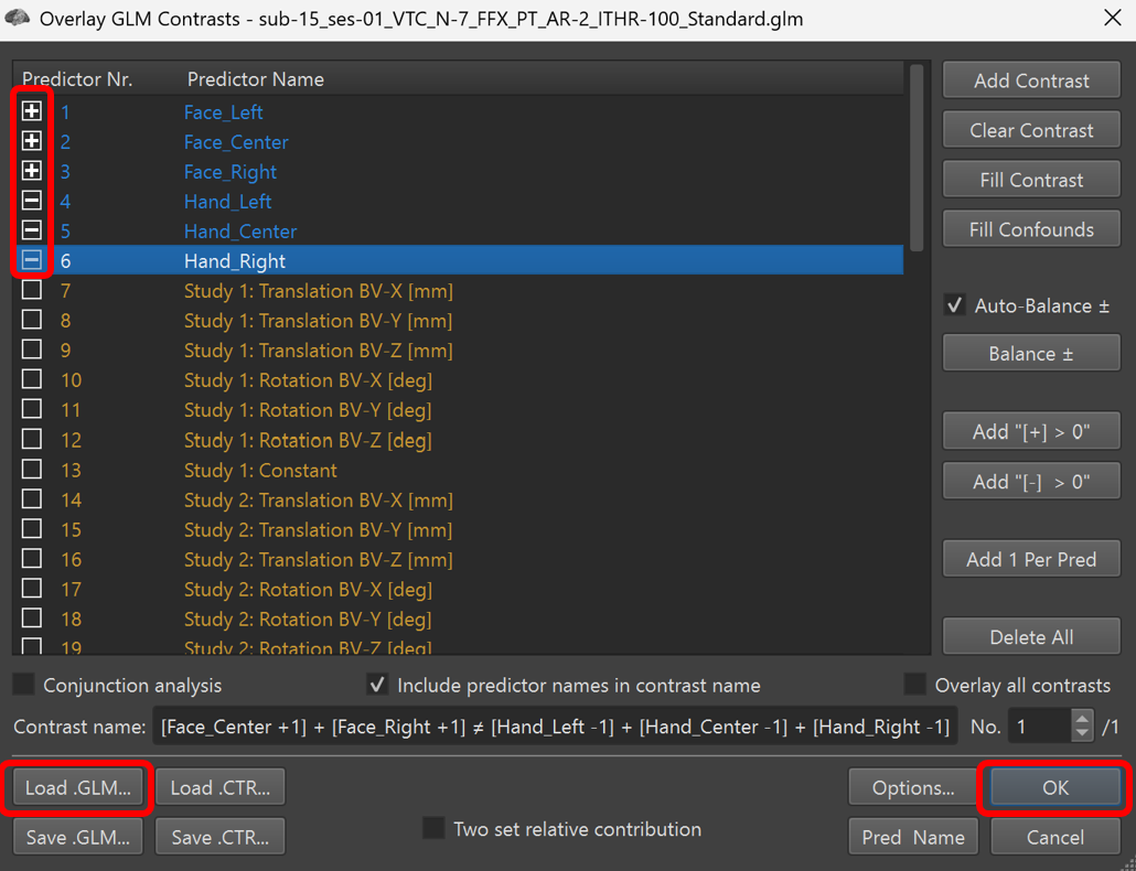
Figure 7-7. A contrast of all three face conditions vs. all three hand conditions in the experimental runs.

Figure 7-8: Activation for the contrast of Faces - Hands. Crosshairs are centred on hand-selective activation in the expected location of LOTChand
Let's explore the the data from one area - the Left LOTChand . One independent way to define a region is to use a web site called neurosynth.org. This site performs meta-analyses of a huge number of published fMRI studies to find which brain regions are most associated with different topics. We did a neurosynth search for "hands" and picked a sphere (7-mm radius) centered around the hotspot in LOTC, which we can call LOTChand.

Figure 7-9. A 7-mm diameter spherical region interest centred on the hotspot of activation for “hands” in Neurosynth. Note the excellent correspondence with the experimental activation in Figure 7-8.
5) Select Analyses/Region-of-Interest Analysis and Load neurosynth_radius_7mm.voi. Select Left LOTChand... and click show VOI . Load one of the experimental time courses in the right side and click Show time course .
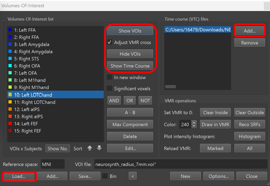
Figure 7-10. Selecting Left LOTChand as a region of interest.
6) Click the small green box in the lower left of the black time course window to expand your options. Now find the Event-Related Averaging box and use browse to select NFs-7_NCs-6_Pre-2-Post-16_PSC-1-BL-From--2-To-0_Bars-SEM_Data-VTC.avg
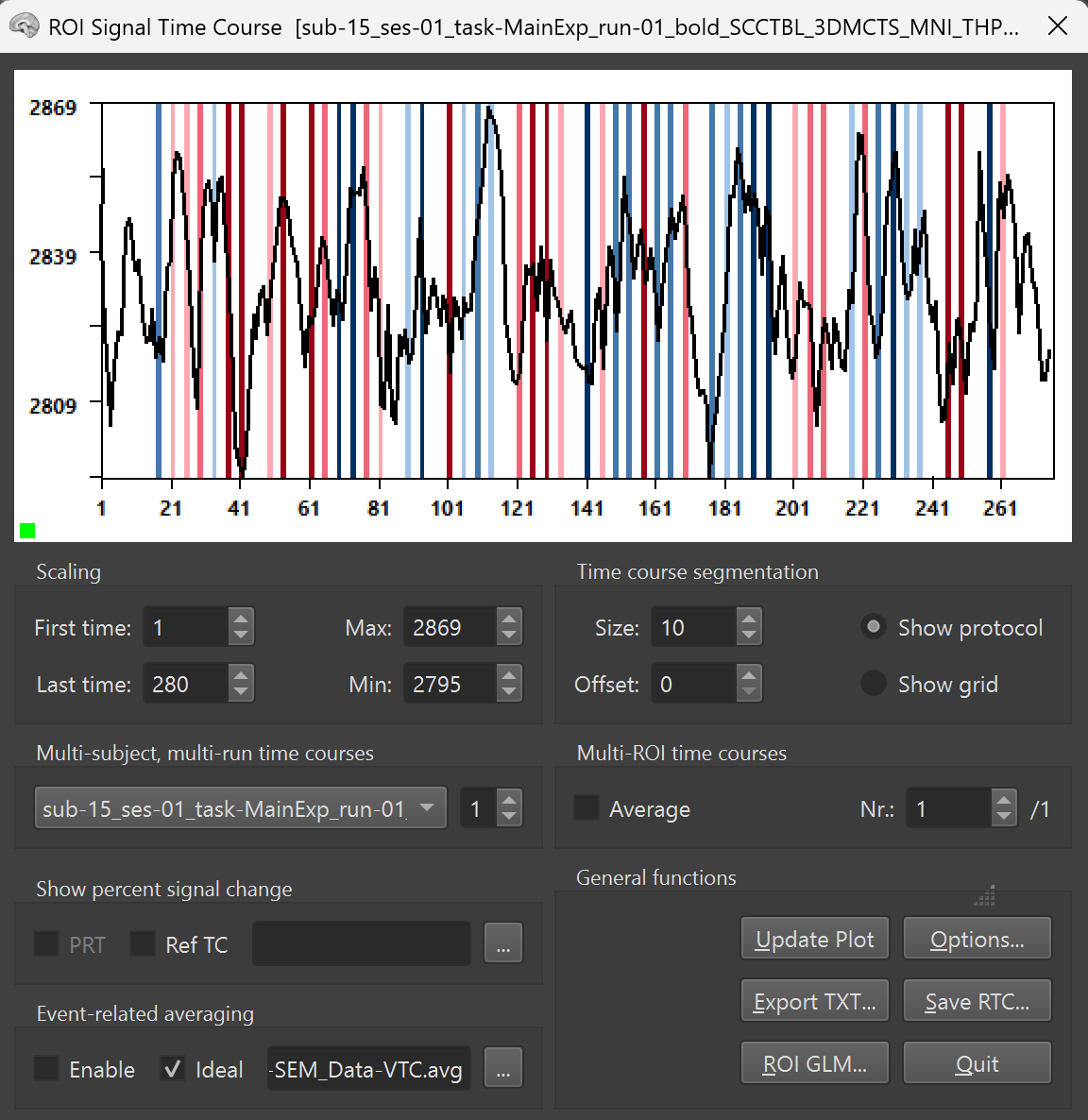
Figure 7-11. Loading the file to generate an event-related average for the region used to extract the time course.

Figure 7-12. The event-related average from Left LOTChand.
Event-related averaging computes the average time course across a window of time for each event. Here, the time window we selected began 2 s before the trial onset and continued for 16 s after. We used file-based averaging to set y=0 to be the average of 18 data points = 3 time points (-2 to 0) for 6 curves. You can see that the curves for the 6 conditions overlap reasonably well here, suggesting that we did a decent job in counterbalancing for order history. You can see that, as expected based on the HRF, the activation peaks about 4 s after the stimuli appeared and the activation in our data is higher for Hands (in green) than Faces (in pink), as one would expect for LOTChand. Data from this time window were extracted for each trial of a given condition, for example, the darkest green time course is the average time course for 56 trials (8 trials/run x 7 runs) of the Hand Left condition.
Question 2:
a) Why do you see a bump every ~4 s in the event-related average?
b) What is the problem with event-related averages when events are densely packed?
DO NOT CLOSE this window since we want to compare later to the output from the deconvolution approach
2. DECONVOLUTION GLM APPROACH
Now that we've seen how the Classic GLM Approach can be applied, let's look at the Deconvolution GLM Approach. One key benefit of the deconvolution approach is that we do not have to assume an HRF and thus we don't have to worry about how errors in the HRF can interact with trial history to yield inaccurate beta weights. Rather, we can use the many repetitions of a given trial type to estimate the best-fit time course for that event by fitting a series of stick predictors to the data. A second key benefit of the "decon" approach is that we can do a much better job at Estimation of the time course of an event type.
Before we use deconvolution on our course experimental data (rapid event-related design with 6 conditions), let's use a simpler example with some simpler localizer data (block design with two conditions). Before (in Tutorial 2), you worked with this data using the Classic GLM Approach. You fit the data using two beta weights, one for an HRF-convolved Faces predictor and one for an HRF-convolved Hands predictor. Feel free to revisit Tutorial 2, 3rd interactive slider section, if you need to refresh your memory.
Now we're going to fit the same data with a deconvolution approach. Instead of 2 predictors, one per condition, plus a constant you'll use 50 predictors (25 per condition), plus a constant. Each of those 50 predictors is a "stick predictor" that estimates the magnitude of activation for a single volume at a particular point in the trial. For example, in this data, in which we sampled the brain every second (TR=1), the 5th predictor for Faces estimates the activation 5 s after the face block began.
Open and play around with the following interactive animation. (Note: if you have trouble opening the animation, please see our troubleshooting page.) Try to adjust the stick predictors to fit the timecourse. Note that adjusting the beta sets the same magnitude for a given time point within each block. Once you realize this is really hard and boring, let the computer do the work for you. Click "Optimize GLM" Note: As this is quite a lot of processing the figure might take a minute or two to finish loading Observe how the stick predictors are adjusted to fit each condition. Note: for consistency with Tutorial 2, this is raw (unpreprocessed) data and the quality of our fit would improve with preprocessing (especially linear trend removal).

Widget 7-1. Fitting a deconvolution model
Question 3: If you exported the 25 beta weights for Faces and the 25 beta weights for Hands, and plotted them in Excel, what would it look like? HINT: Look at the profile of the sliders after optimization.
Deconvolution on Example Data
Now, you should have a better understanding of how deconvolution works so we can apply it to our experimental runs, which used a jittered rapid event-related design.
1) Open a second copy of the vmr (sub-15_ses-01_T1w_IIHC_MNI.vmr) in a new window/tab and link the same vtc file (sub-15_ses-01_task-MainExp_run-01_bold_SCCTBL_3DMCTS_MNI_THPGLMF3c_SD3DVSS8.00mm.vtc) again.
Use the Window/Tile command and the "Link VMRS" tick box in blue box mode to enable you to see the same locations in your two VMRs.
- In order to make deconvolution predictors instead of our regular convolved predictors, click on your new VMR window to make sure it is the active one and then open GLM Single-Study (Analysis tab), click options and choose Deconvolution Design , then Define Predictors. Now inspect these predictors by stepping through them in the Predictors section of the window.
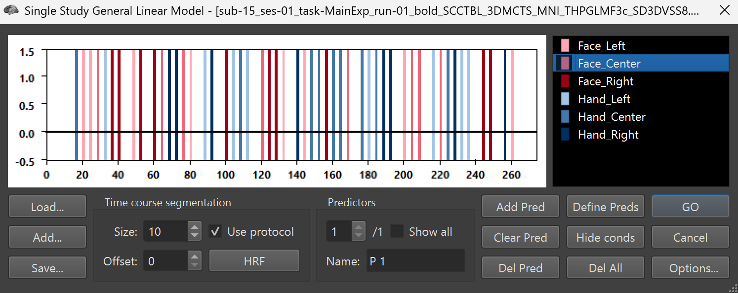
Figure 7-13. To access the menu for a deconvolution design, go into Options.
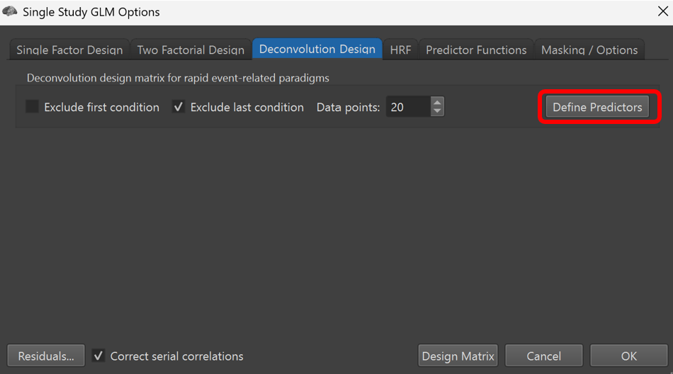
Figure 7-14. The options tab for a deconvolution analysis.
We have 20 predictors/condition x 6 conditions = 120 predictors. Why 20/condition? We know that it takes up to ~20 s for the hemodynamic response to return to baseline after a brief stimulus so we want to model the full time span. Here we collected one volume every 1 s (i.e., TR = 1 s) so 20 predictors/condition is appropriate.
Question 4: If we were to repeat the experiment with a TR = 0.5 s, how many predictors in total (for all conditions) would we want?
We already generated a deconvolution design matrix for each run and made a .mdm and .glm that you can now examine.
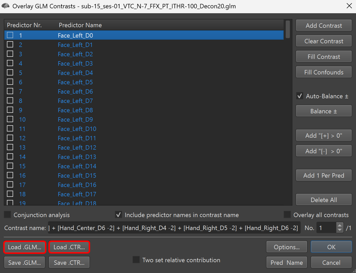
Figure 7-15. The GLM output for the deconvolution analysis has 120 predictors of interest. For complex contrasts, a .ctr file can be loaded.
3) In the analysis tab go to overlay General Linear Model... and load this file sub-15_ses-01_VTC_N-7_FFX_PT_ITHR-100_Decon20.glm
You will now see several predictors for each condition instead of just one per condition. But how are we going to do a contrast with this many predictors? Instead of contrasting all these predictors with each other we will only contrast the "peak responses" . With a stimulus that lasts about 2 s, we usually expect the peak to occur somewhere between predictors 4,5 or 6 so we will only compare these predictors across conditions: +Faces_Left456 +Faces_Center456 +Faces_Right456 -Hands_Left456 -Hands_Centre456 -Hands_Right456).
We already set this contrast up for you in a CTR file.
4) In the open window find Load CTR... and load Decon_F456-H456.ctr and click OK
Compare the contrast from the Classic GLM in the beginning of this tutorial for +F-H to the contrast from deconvolution GLM with +F456-H456. Make sure to set both maps to the same statistical threshold (e.g., t>6) under Analysis/Overlay Volume Maps/Statistics tab/Use statistic value/change confidence range to minimum = 6
Question 5: Why not do a contrast with all 60 Face predictors set to + and all 60 Hand predictors set to -?
Question 6: How similar do the maps look? What differences can you find? In sum, how well does the deconvolution approach work for detecting activation blobs?
Now let's see what the deconvolved time course looks like...
Now we can estimate the time course a the same region that we used earlier, e.g., LOTChand defined by neurosynth on "hands".
In the VMR window that you used for deconvolution (you can now close the VMR window with the classic approach now)...
5) Go to Analysis / Region-of-Interest Analysis and Load the neurosynth_radius_7mm.voi. Select the Left LOTChand... and Show VOI . In the Options menu under the Access Options tab, click Browse Design Matrix and load the file sub-15_Decon20_MotionPONI_FFX.mdm
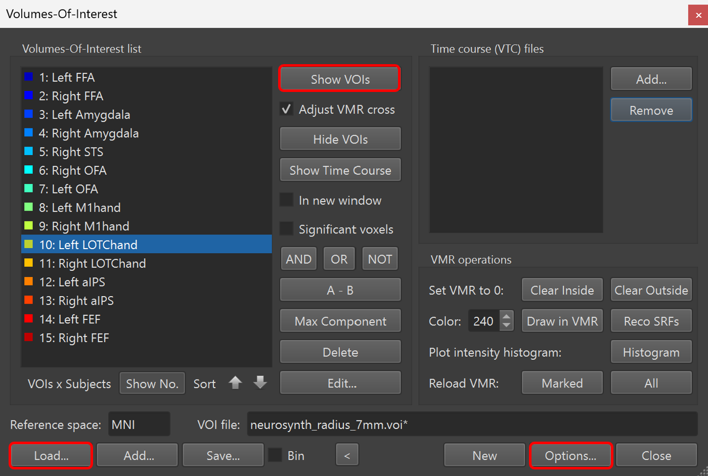
Figure 7-16. Selecting the LOTChand ROI.
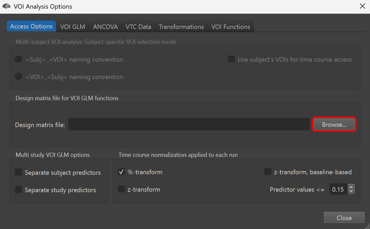
Figure 7-17. Loading the deconvolution design matrix.
In
VOI GLM
tab, select Left LOTChand and create GLM output (table/plot) for selected VOI.
Now click in the same window
VOI GLM
and you will see a window pop up.
Press
Fit GLM
and look at Event-related Deconvolution Plot.
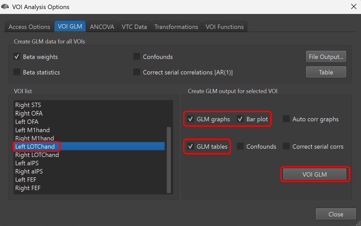
Figure 7-18. Running a deconvolution analysis for the LOTChand ROI.
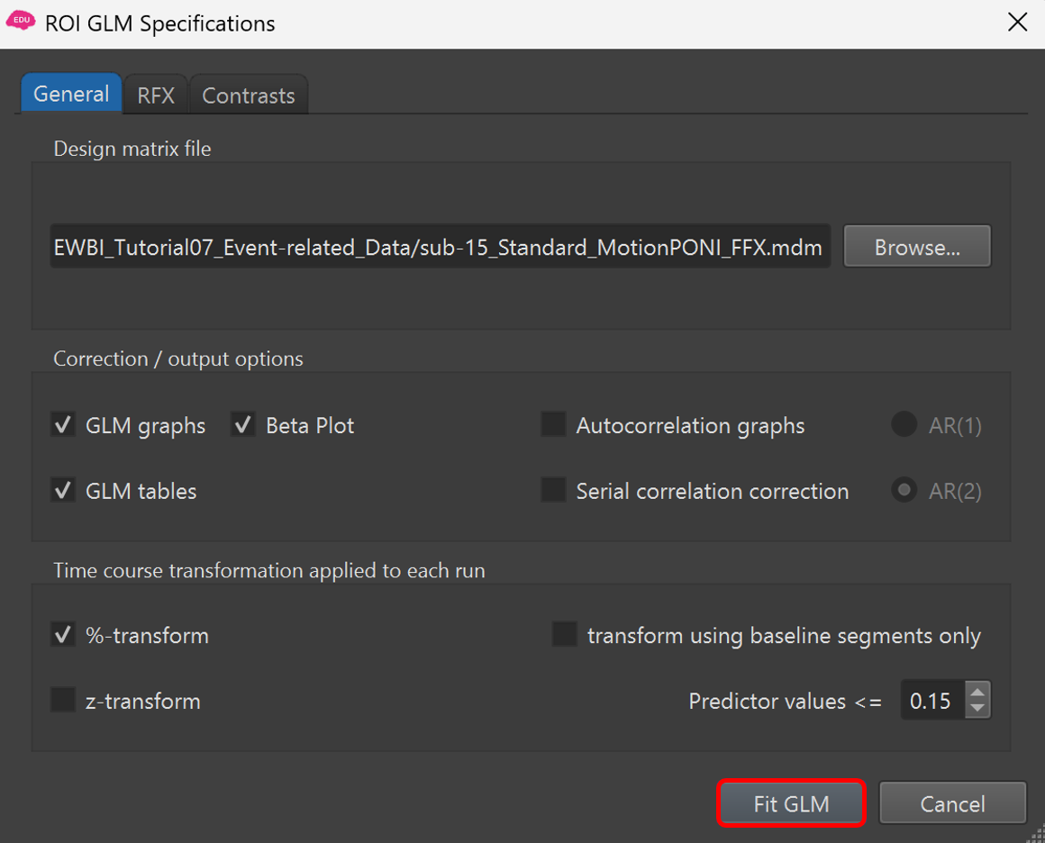
Figure 7-19. Options to select for Fitting the GLM.
Question 7: How does the deconvolution plot look different from event-related average? Why?
Question 8: Does this participant have a default HRF shape? What would be the consequences for this plot and for the differences between the classic and deconvolution maps if they had an individual HRF that was very different from the default HRF shape?
Question 9: What are the pros and cons of deconvolution vs. classic GLM approaches for rapid event-related designs? When is deconvolution most worthwhile?