Tutorial 6 - fMRI Preprocessing & Quality (Spatiotemporal Smoothing)
Goals
To become familiar with a variety of spatial and temporal smoothing methods
To understand how to assess the statistical impact of preprocessing steps in a single run
Relevant Lectures
Lecture 04c: Preprocessing and Predictors of No Interest
Lecture 04d: Preprocessing
Accompanying Data
Background
fMRI data is noisy by nature – both spatially and temporally. Spatial noise is often a concern for anatomical images because noise across different voxels can make the images look grainy and make it harder to discern tissue types (e.g., gray vs. white matter). Temporal noise is especially relevant for functional MRI. Temporal noise refers to changes in signal intensity over time that are due to factors other than the BOLD response to our protocol.
Temporal variability can arise from physical noise, especially on low-field scanners (e.g., 1.5T) or scanners that do not undergo regular quality assurance testing. Temporal variability can also arise from physiological noise, which includes factors related to the participant such as head and body motion, breathing and cardiac pulsations, as well as performance factors such as fluctuations in alertness.
To increase the signal-to-noise ratio, several strategies are available. You have already seen in Tutorial 4 how motion correction can typically, but not always, reduce noise. Even when correction is not fully successful, including motion parameters as predictors of no interest can "soak up" variance due to motion and thus improve statistics.
In this tutorial, you will examine two additional preprecessing steps that can improve signal-to-noise: spatial smoothing and temporal filtering preprocessing steps.
Conceptual Refresher – Spatial Smoothing
During spatial smoothing, for each volume (time point), each voxel’s intensity is computed as a weighted average of its own intensity and the intensities of its neighbours within a set radius. The closer the neighbouring voxel, the more it contributes to the new intensity. The weights are determined by a Gaussian function and its size is characterized by its width at a y-value = half its height, which is called the full width at half maximum (FWHM) of the smoothing kernel (Figure 6-1).
If the noise is at a finer spatial scale than the signal, spatial smoothing improves data quality because genuine differences in intensity summate while noise differences cancel out. See Figure 6-2.

Figure 6-1. A Gaussian filter is characterized but the full-width at half maximum (FWHM).

Figure 6-2. The BEFORE photo shows a grainy image that is due to noise related to taking a photo in dim light. The AFTER photo shows how spatial smoothing can make the picture look better. Adjacent pixels share differences in intensity (e.g., the cloud pixels are darker than sky pixels) but noise also leads to speckles (more fine-scale differences in intensity). When intensity levels for each pixel are smoothed through a weighted combination with neighboring pixels, differences in signal reinforce one another (e.g., dark cloud pixels are combined with other dark cloud pixels; light with light) while differences due to noise cancel one another out (a noisily bright pixel will be next to other pixels with lower intensities). Photo credit.

Figure 6-3. One functional data slice with different smoothing options.
Figure 6-3 shows a slice of functional data without smoothing (left), with 4-mm FWHM smoothing (centre), and with 8-mm FWHM smoothing (right). Notice the effects of the increasing the smoothing kernel. Note that some smoothing (4 mm) blurs out the speckles, making it easier to see gray vs. white matter differences while heavier smoothing begins to blur out gray and white matter together.
Spatial smoothing is also beneficial for reducing temporal noise. Adjacent voxels likely share temporal signal (e.g., a voxel that responds strongly when faces are shown is likely to be next to other voxels with a similar preference) but not temporal noise (especially physical noise). Spatial smoothing makes time courses cleaner because signals reinforce one another while noise cancels.
Instructions: Spatial Smoothing
We have taken one run of the Localizer from one participant and applied different levels of spatial filtering to the data. We have also selected a peak voxel in the FFA and LOTC hand regions of interest. You will examine the maps to see how the data are affected by different types of filtering.

Figure 6-4. A file with multiple maps of the same contrast (Faces - Hands) after different combinations of spatial smoothing and temporal filtering.
1) Select File/Open, and open the anatomical file sub-03_ses-01_T1w_IIHC.vmr
- Select Analysis/ Overlay Volume Maps, and then load SpatialSmoothing_multimap.vmp. Note: A .vmp (for volumetric map) is a data format that allows you to save, load, and combine maps from different contrasts.
You will see that 6 maps have been created for you. All of these maps have been generated from a contrast of (+1 x Faces) + (-1 x Hands) such that face-selective areas will appear in the orange-yellow spectrum and hand-selective areas will appear in the blue-green spectrum (if you are using the classic look-up table... if not, you can change the lookup table under the menu, BrainVoyager/Preferences... Default map lookup table = Classic map colors (pre-21).
All of the maps have been set to the same statistical cutoffs (minimum t = 3; maximum t = 6) to enable "apples to apples" comparisons between maps. You may wish to uncheck "Interpolate" if you want to more accurately visualize the voxels that the maps are actually based upon. Pay attention to the first four maps for now. These are an unfiltered run (with slice time - SCCTCBL - and motion - 3DMCTS - correction) and three levels of spatial smoothing (SS4, SS8, and SS12, where the number indicates the FWHM of the Gaussian kernel).
3) Toggle between the first four maps by clicking the box to the left of the map name until a plus sign appears beside the map you want to view. Pay particular attention to regions around the expected location of FFA and LOTC (Hint: A good slice to look at is y = 178, where you can see both areas in both hemispheres). hand as well as to the "schmutz" (voxels that are in regions where no BOLD signal is possible/likely).
Question 1:
a) What effect does spatial smoothing have on the appearance of the maps?
b) Which of the two brain regions (FFA and LOTChand) is larger? How does the optimal smoothing kernel size differ for the two brain regions? Based on this, how should the expected size of targeted brain regions affect the choice of smoothing kernel (matched filter theorem)?
c) Is more smoothing necessarily better? Select all that apply.
- More smoothing is always better.
- More smoothing can remove spurious activation like lone voxels that are active purely due to chance.
- Too much smoothing can eliminate legitimate activation in small blobs.
- Some smoothing can enhance activation in blobs that are similar in size to the smoothing kernel.

Figure 6-5. How to load an ROI/VOI file.
- Now let's compare how spatial smoothing affects the time course of single voxels. Select Analysis/Region-of-Interest Analysis and load FFA+LOTChand+noise.voi. This file contains the spatial locations of two voxels, one in FFA and one in LOTChand . By defining each voxel as a region of interest, we can ensure that, as you inspect different time courses, they will be based on the same voxel. For each voxel, you can select the name and then click "Show VOIs". As you do so, the crosshairs will jump to that voxel's location in 3D space. (Note that the left side of the ROI dialog box has a list of files under Time Course (VTC) files.) Unfortunately because of the way BrainVoyager stores file paths, the paths will be incorrect for your data. Remove each of the files and add them in the following order - you might not see the vtc files - in this case just add the vtc files one at a time.
- sub-03_ses-01_task-Localizer_run-01_bold_SCCTBL_3DMCTS_256_sinc3_2x1.0_NATIVE.vtc
- sub-03_ses-01_task-Localizer_run-01_bold_SCCTBL_3DMCTS_256_sinc3_2x1.0_NATIVE_SD3DVSS4.00mm.vtc
- sub-03_ses-01_task-Localizer_run-01_bold_SCCTBL_3DMCTS_256_sinc3_2x1.0_NATIVE_SD3DVSS8.00mm.vtc
- sub-03_ses-01_task-Localizer_run-01_bold_SCCTBL_3DMCTS_256_sinc3_2x1.0_NATIVE_SD3DVSS12.00mm.vtc
For the voxels in FFA and LOTChand, step through each of the first four time courses (NATIVE, FWHM = 4; FWHM = 8; FWHM = 12).
Question 2:
a) Mathematically, what happens to a time course whe we apply spatial smoothing?
- Activation is averaged across neighboring time points.
- Activation is averaged across neighboring voxels.
- Activation is averaged across the entire brain.
- Activation does not exist.
b) Why do time courses "look better" when the right amount of smoothing compared to no smoothing? Why do time coureses "look worse" when too much smoothing is applied?
Question 3: For each situation, indicate whether and how much you would want to spatially smooth the data?
- When the region of interest is large.
- When the region of interest is very small.
- When the native voxel size is relatively large and the scanner has moderate SNR (e.g., 3 mm isotropic at 3T).
- When the native voxel size is relatively small and the scanner has high SNR (e.g., 0.5 mm isotropic at 7T).
- When multivoxel pattern analysis (MVPA) is being used to analyze the data.
- Forshadowing for Group lecture and tutorial: When group data are being analyzed with a voxelwise analysis in MNI space.
Conceptual Refresher – Temporal Filtering
Using Fourier analysis, any time series (such as an fMRI time course) can be broken down into a series of sine waves. This is very useful for time series analyses because different sources of noise can occur cyclicly predominately in particular frequency bands. For example, outdoor temperature as a function of time (say over 20 years) would show cycles related to time of day (1 cycle/24 hours), time of year (1 cycle per year), and long-term climate changes (slow drifts), in addition to ~random fluctuations related to everyday weather.
fMRI data tends to have high noise in particular frequency ranges:
Very low frequencies related to scanner drift and participant relaxation
Frequencies related to breathing: ~0.3 Hz = 0.3 cycles/s [to calculate the period of a sine wave, take 1/frequency: (1/(0.3 cycles/sec)) = 3.3 s/cycle]
Frequencies related to heart rate: ~1 Hz = 1 cycle/sec [= 1 s/cycle = ~60 beats/min]
Geek note: You can only see these frequencies if you have a TR of ~0.5 s or faster (due to a principle called the Nyquist limit) so most fMRI studies will miss them
The expected activation for a paradigm can also be dominated by particular frequencies.
In an optimal experiment, the paradigm frequencies will have little overlap with the noise frequencies.

Figure 6-6. For simple two-condition protocol, it is easy to predict the predominant frequency of activation.
In addition, good fMRI data will have legitimate BOLD signals at the frequency (or range of frequencies) of the paradigm. For simple designs (off-on-off-on…), as shown in Figure 6-3, this is easy to calculate. For example, if you have a run of 340 s with 16-s periods of off and on, you would have 10.5 cycles/340 s (Note, the extra half cycle comes from the baseline period at the end; if it ended at the end of the last pink cycle, there would be exactly 10 cycles). To compute the expected stimulation frequency in Hz: 10.5 cycles/340 s = 0.03 Hz.

Figure 6-7. Expected activation after HRF convolution.
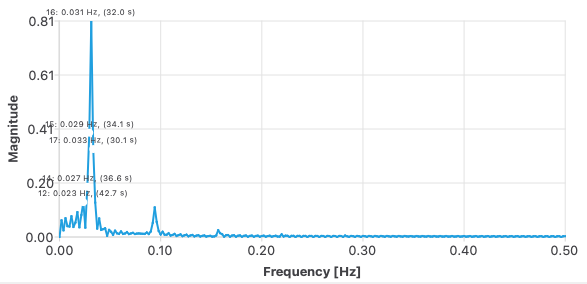
Figure 6-8. Fourier spectrum of the time course shown in Figure 6-7
Geek note: Because the expected shape of the activation is not a pure sine wave, you might also expect stimulation-related signal at the harmonics = integer multiples of the main (fundamental) frequency, e.g., 0.06 Hz, 0.09 Hz, etc.)

Figure 6-9. For more complex, multi-condition protocols, the expected stimulation frequencies may be more complicated.
For designs such as the localizer data (Figure 6-7), which do not have precisely consistent periods (e.g., the time between the first and second pink epochs is shorter than the time between the second and third ones), you would not expect such straightforward paradigm-related frequencies. Nevertheless, since we have 4.2 cycles of stimulation for each condition, you would expect stimulus related activation to be around 4.2 cycles/340 s = ~0.012 Hz.
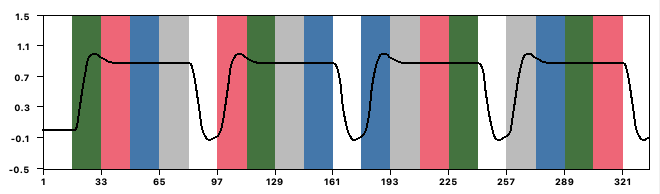
Figure 6-10. The expected activation for a region with an equivalent visual response across all four stimulus conditions compared to baseline.

Figure 6-11. Fourier spectrum of the time course shown in Figure 6-10.

Figure 6-12. The expected activation for a region with a response to faces.

Figure 6-13. Fourier spectrum of the time course shown in Figure 6-12.
One strategy for improving fMRI statistics is to filter out frequencies outside of the expected paradigm frequencies. By removing noise at these frequencies, the residuals become smaller and thus our statistics improve.
Voxel (and region) time courses can also be subject to Fourier analysis. This can reveal energy at paradigm frequencies as well as energy at noise frequencies.

Figure 6-14. Time course from a voxel in LOTChand.

Figure 6-15. Fourier spectrum of the time course shown in Figure 6-14.

Figure 6-16. Time course from a voxel with low-frequency drift

Figure 6-17. Fourier spectrum of the time course shown in Figure 6-16.
Instructions: Temporal Filtering
Question 4. What differences do you see in the Fourier plots in Figures 6-15 and 6-17? Why would such differences exist?
This is the protocol for the data above. Pink is Faces and Blue is Hands. Each Face, Hand and Baseline epoch lasted 16 s.
Question 5: What is the expected frequency for fluctuations related to visual stimulation, expressed both in cycles/run and in Hz? What is the expected frequency for fluctuations related to face-specific responses, expressed both in cycles/run and in Hz?
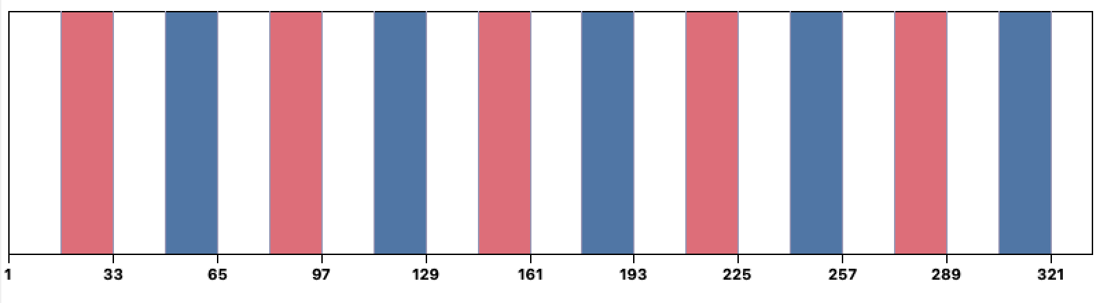
Figure 6-18. Example protocol with three conditions, Faces (in pink), Hands (in purple) and baseline (in black).
Linear Trend Removal
The simplest temporal filtering we can do is to filter out any linear drifts in our data. In Tutorial 2 (Question 3), you saw that after we fit a GLM to our raw data, one of the main sources of residual error was due to linear drift.
Widget 6-1 allows you to "fix" linear trends in two ways. Let's look at the GLM without either correction, with correction through linear trend removal (preprocessing), and with the linear trend removed through a PONI.

Widget 6-1. How linear trend removal affects the GLM.
5) Use only the leftmost slider and the constant slider (keep the PONI slope at zero) to approximate the best fit beta weights for Voxel B when the linear trend is uncorrected. Note the appearance of the residuals and the magnitude of the sum of squared error.
Next, go back to the data above. Turn on "Linear Trend Removal" and re-fit the GLM . You can do this manually or use the Optimize GLM button. Note the appearance of the residuals and the magnitude of the sum of squared error.
Next, turn off "Linear Trend Removal" and re-fit the GLM, including the PONI slope slider . You can do this manually or use the Optimize GLM button. Note the appearance of the residuals and the magnitude of the sum of squared error.
Question 6:
a) How did the residuals and squared error change after linear trend removal? Was one approach to dealing with linear trends better than the other?
b) Considering the relationship between statistical power, the variance accounted for by our model and the variance left over (residuals), why is temporal frequency filtering beneficial?
High Pass Filtering
We can filter out the lowest temporal frequencies in our data, allowing the high frequencies to pass through the filter (hence the term high-pass filtering). Software defaults will typically filter out changes slower than 2-3 cycles/run (These values in Hz will depend on your run duration and will be very slow, e.g., 3 cycles/340 s = 0.009 Hz). High pass filtering also filters out linear trends so adding linear trend removal is redundant (You can think of a linear trend as being an ultra-low frequency -- imagine a sine wave wider than your screen with the upward or downward slope crossing though your time course).
Low-pass Filtering (aka Temporal Smoothing)
We can filter out the highest temporal frequencies in our data, allowing only the low frequencies to pass. One way to to this is to smooth the time course data with a Gaussian kernel over time. This technique is very similar to Gaussian spatial smoothing. This is why you may also hear it called temporal smoothing. A smoothing kernel is applied over each time point in a voxel’s time course. But instead of computing the weighted average of neighbouring voxel intensities at the same time, temporal smoothing computes those averages over time, using neighbouring time points. The following shows a voxel time course with no smoothing (top), 1 time point smoothing (centre), and 2 time point smoothing (bottom).
As you will see, low-pass filtering is typically NOT recommended in fMRI because it exacerbates the problem of serial correlations (temporal autocorrelation).

Figure 6-19. I hate this figure. Need to replace it.
Band-pass Filtering
If we filter out both low frequencies and high frequencies, we are allowing only an intermediate band of frequencies to pass through. Generally bandpass filtering is NOT recommended for the same reason that low-pass filtering is NOT recommended. Nevertheless, you may see papers that discuss this so it is useful to understand what it means.
The following is an interactive widget to explore band-pass filtering. Two sliders, Minimum Freq. and Maximum Freq. have been added to control which frequency components are allowed to contribute to the signal. To perform high-pass filtering, set the minimum frequency to remove frequencies below that value. To perform low-pass filtering, set the maximum frequency to remove frequencies above that value. To do band-pass filtering, set minimum and maximum frequencies to remove frequencies at either extreme. (Note: if you have trouble opening the animation, please see our troubleshooting page)

Widget 6-2. How temporal filtering affects the GLM.
8) In the widget, Fit the GLM (use Optimize GLM if you like) for Voxel 1 and note the beta weights, squared error, and pattern of residuals. Adjust the Minimum Freq slider to 0.01 Hz (without adjusting the Maximum Freq slider just yet). This means you are filtering out any frequencies below 0.01 Hz (and passing any frequencies above that cutoff). Refit the GLM and again note the beta weights, squared error, and pattern of residuals.
Question 7: What effect did this have on your data and what would be the consequences to your statistical significance?
- Now try higher values for the minimum frequency (e.g. 0.1 Hz) and refit the GLM to see what effect it has.
Question 8: What are the consequences of aggressive high-pass filtering and why? What would be an optimal cuttoff for this protocol?
10)
Set the Minimum Freq
to the value you think is
most appropriate
here.
Now see what effect changing the Maximum Freq has on your data and model fits. The maximum frequency our data can have is 1 Hz because we sampled with a TR = 1 s, so we cannot filter out a Maximum Freq > 1 Hz.
Question 9: Fill in the blanks: Changing the maximum frequency makes the time course (smoother/noisier). However, this also (increases/decreases) the temporal autocorrelation which is (good/bad) from a statistical point of view.
Question 10: Based on your answer to Question 9, what is considered best practice for temporally filtering fMRI data? a) High-pass filtering only; b) Low-pass filtering (i.e., temporal smoothing) only; c) Bandpass filtering?
Question 11: What happens if you set both Maximum Freq and Minimum Freq to 0.1 Hz? Why?
11) In Brain Voyager, use Analysis/Overlay Volume Maps to load TemporalFiltering multimap 2025-11-12.vmp. Toggle between the three maps, which have the same spatial smoothing (FWHM = 4 mm) but different temporal filtering settings applied to them.
Question 12: What effect do the added steps have on the statistical maps? Why? Why wouldn't you want to use the map that looks the "most significant"?
Optional: If you want to see the effect of the temporal filtering steps on the time course appearance, use Analysis/Region-of-Interest analysis to load FFA+LOTChand+noise.voi. Expand the window and Add the following .vtc files:
• sub-03_ses-01_task-Localizer_run-01_bold_SCCTBL_3DMCTS_256_sinc3_2x1.0_NATIVE.vtc
• sub-03_ses-01_task-Localizer_run-01_bold_SCCTBL_3DMCTS_256_sinc3_2x1.0_NATIVE_SD3DVSS4.00mm_THPGLMF3c.vtc
• sub-03_ses-01_task-Localizer_run-01_bold_SCCTBL_3DMCTS_256_sinc3_2x1.0_NATIVE_SD3DVSS4.00mm_THPGLMF3c_TDTS2.8s.vtc
Then for the three voxels, click the vtc you want to see and then click "Show Time Course"