Tutorial 3 - Understanding the General Linear Model (GLM)
Goals
To develop an intuitive understanding of the how the General Linear Model (GLM) is used for univariate, single-subject, single-run fMRI data analysis
To understand different components of the GLM, including the beta weights, predictors, residuals
To understand what is the optimal number of predictors and why baseline predictors are redundant
To understand statistical significance of beta weights in time course analyses
To learn how to use contrasts in statistical analyses
Relevant Lectures
Lecture 03c: fMRI statistics: Extending the GLM to more conditions and multiple runs
Accompanying Data
Background and Overview
In the previous of the tutorial, we discussed how we can use correlation to know whether a voxel reliably activates to a certain stimulus. However, that does not inform us on how activated the voxel is. Luckily, other familiar statistical techniques can be used to estimate these levels of activation. For example, you can extract an estimate of how active the voxel or region was in different conditions and then simply perform a t-test to examine whether activation levels differ between two conditions. Alternatively, if you have a factorial design, such as our Main Experiment, which tested Faces/Hands Categories x Left/Centre/Right Directions (a 2 x 3 design), you can run an ANOVA to look for main effects and interactions. All of these common statistical tests can be applied through a General Linear Model (GLM). The GLM is the "swiss army knife" of statistics, allowing you to accomplish many different goals with one tool.
I. Applying the GLM to Single Voxel Time Courses
Beta Weights, Residuals and the Best Fit
The GLM can be used to model data using the following form: y = β0 + β1X1 + β2X2 + ... + βnXn + e where:
- y is the observed or recorded data,
- β0 is a constant or intercept adjustment,
- β1 ... βn are the beta weights or scaling factors
- X1 ... Xn are the independent variables or predictors.
- e is the error (residuals).
In the case of fMRI analyses, you can think of this as modelling a data series (time course) with a combination of predictor time courses, each scaled by beta weights, plus the "junk" time course (residuals) that is left over once you've modelled as much of the variance as you can. These three components of the GLM are illustrated for a simple correlation in the figure below.

Figure 3-1. Here the GLM is used for the simplest possible situation, a correlation.
Using this model, we can try to find the best fit. The best fitting model is found by finding the parameters (beta weights and constant) that maximizes the explained variance(signal), which is also equivalent to minimizing the residuals.
Question 1: Match the following terms to the appropriate formula symbols.
- Y 1. Residual/error
- B0 2. Predictor function
- B1 3. Beta/slope
- X1 4. Time course data from the voxel
- E 5. Constant/intercept
Estimating Beta Weights
In the following animation, adjust the sliders until you think you have optimized the model for Voxel A (i.e., minimized the squared error). Make sure you understand the effect that the four betas and the constant are having on your model. You can test how well you did by clicking the Optimize GLM button, which will find the mathematically ideal solution.

Widget 3-1. Fitting a 4-POI GLM to the localizer data from 3 voxels
Question 2:
a) How can you tell when you've chosen the best possible beta weight and constant? Consider (1) the similarity of the predictors (pink, blue, green, purple) and the data (black) in the top panel; (2) the appearance of the residual plot in the bottom panel; and (3) the squared error and sum of residuals?
b) What can you conclude about Voxel A's selectivity for images of faces, hands, bodies and/or scrambled images?
- Voxel A is specifically selective to hands and faces
- Voxel A is specifically selective to bodies and scrambled
- Voxel A is specifically selective to hands, faces and bodies
- Voxel A is not specifically selective to any of the 4 types of stimuli
c) Do the same for Voxel's E and F. What can you conclude about their selectivity for images of faces, hands, bodies and/or scrambled images?
- Voxel E is selective to hands and Voxel F is selective to faces and bodies
- Voxel E is selective to faces and Voxel F is selective to hands and bodies
- Voxel E is selective to faces and Voxel F is selective to hands only
- Voxel E is selective to hands and Voxel F is selective to faces only
d) Define what a beta weight is and what it is not. In other words, what is the difference between a beta weight and a correlation coefficient?
What about the baseline?
You might have noticed that our models only have predictors for conditions and none for the baseline, and you might be wondering why that is. To explain this, let's go back to basic agebra.
Imagine you trying to find the value of x in the following equation: 2x + 3 = 5. You might have guessed the answer is x = 1.
Now imagine you are trying to find x for the following equation: 2x + 3y = 5. In this case, there are an inifinite number of solutions, making it hard to know which is the correct one! Adding an extra variable makes the equation unsolvable.
If we use the same number of predictors as there are conditions, we have similar problem with time courses in fMRI analyses. In other words, having an equal number of conditions and predictors makes the model redundant. Let's try it out.

Widget 3-2. The effect of erroneously including a redundant baseline predictor. To make the two predictors completely redundant, we used the unconvolved (box car) versions of the predictors. The redundancy would be slightly less with convolved predictors; nevertheless, redundancy would be suboptimal.
Adjust the sliders for the visual & baseline predictor model (left) until you think you have optimized the model while keeping the constant at 0. Then, click on the optimize GLM button.
Question 3:
a) What optimal betas did you find for the 2 predictor (visual +baseline) model? Now compare these to the optimal betas for a single visual predictor (right). What do you notice?
- The betas for the baseline model (two predictors) are approximately the same as for the single predictor model.
- The betas for the baseline model (two predictors) are approximately half as large as for the single predictor model.
- The baseline model has one predictor with a beta equal to 0 and another predictor with a beta approximately equal to the beta obtained in the single predictor model.
- None of the above are correct.
b) How many possible combinations of betas and constant are possible for the model with baseline and visual predictors? Why is this suboptimal?
II. Whole-brain Voxelwise GLM in BrainVoyager
In the previous section, we explained how the GLM can be used to model data in a single voxel by finding the best fit (in other words, the optimal beta weights and constant). Now, we can apply this to the whole brain by fitting one GLM for every voxel in the brain.
Conducting a GLM analysis
1) Select File/Open... , open sub-10_ses-01_T1w_BRAIN_IIHC.vmr. Then attach the VTC by selecting Analysis/Link Volume Time Course (VTC) File... . In the window that opens, click Browse , and then select and open sub-10_ses-01_task-Localizer_run-01_bold_256_sinc3_2x1.0_NATIVEBOX.vtc , and then click OK .
2) Select Analysis/General Linear Model: Single Study. By single study, BrainVoyager means that we will be applying the GLM to a single run.
Click options and make sure that Exclude last condition ("Rest") is checked (the default seems to be that Exclude first condition ("Rest") is checked).
3) Click Define Preds to define the predictors in terms of the PRT file opened earlier and tick the Show All checkbox to visualize them. Notice the shape of the predictors – they are identical to the ones we used earlier for in Question 2. Now click GO to compute the GLM in all the voxels in our functional data set.
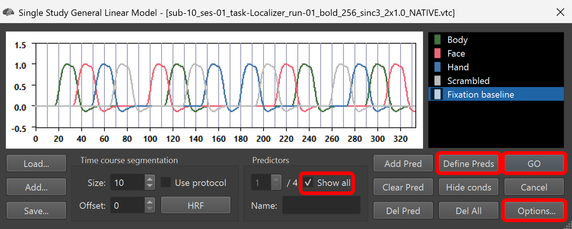
Figure 3-2. Defining predictors.

Figure 3-3. This tab on the Single Study GLM dialog allows you to exclude the baseline condition if it is the first or last condition specified.
After the GLM has been fit, you should see a statistical "heat map" . This initial map defaults to showing us statistical differences between the average of all conditions vs. the baseline . More on this later.
In order to create this heat map, BrainVoyager has computed the optimal beta weights at each voxel such that, when multiplied with the predictors, maximal variance in the BOLD signal is explained (under certain assumptions made by the model). Another, equivalent interpretation, is that BrainVoyager is computing beta weights that minimize the residuals. For each voxel, we then ask, “How well does our model of expected activation fit the observed data?” – which we can answer by computing the ratio of explained to unexplained variance.

Figure 3-4. GLM
It is important to understand that, in our example, BrainVoyager is computing four beta weights for each voxel – one for the Face predictor, one for the Hand predictor, one for the Bodies predictor and one for the Scrambled images predictors. And for each voxel, residuals are obtained by computing the difference between the observed signal, and the modelled or predicted signal – which is simply vertically scaled by the beta weights. This is the same as you did manually in Question 2.
But we don't simply want to estimate activation levels for each condition by computing beta weights; we also want to be able to tell if activation levels differ statistically between conditions!
Comparing Activation between Conditions
Just as with statistics on other data (such as behavioral data), we can use the same types of statistics (e.g, t tests, ANOVAs) to understand brain activation differences and the choice of test depends on our experimental design (e.g., use a t test to compare two conditions; use an ANOVA to compare multiple conditions or factorial designs). Statistics provides a way to determine how reliable the differences between conditions are, taking into account how noisy our data are. For fMRI data on single participants, we can estimate how noisy our data are based on the residuals.
For example, we can use a hypothesis test to test whether activation for the Face condition (i.e., the beta weight for Faces) is significantly higher than for Hands, Bodies and Scrambled images (i.e., the beta weight for Hands, Bodies and Scrambled images). Informally, for each voxel we ask, “Was activation for faces significantly higher than activation for Hands, Bodies and Scrambled images?”
To answer this, it is insufficient to consider the beta weights alone. We also need to consider how noisy the data is, as reflected by the residuals. Intuitively, we can expect that the relationship between beta weights is more accurate when the residuals are small.
Question 4: Why can we be more confident about the relationship between beta weights when the residual is small? If the residual were 0 at all time points, what would this say about our model, and about the beta weights? Think about this in terms of the examples in Questions 1 and 2 from the previous tutorial (Tutorial 2).
We can perform these kind of hypothesis tests using contrasts . Contrasts allow you to specify the relationship between beta weights you want to test. Let's do an example where we wish to look at voxels with significantly difference activation for Faces vs Hands.
4) Select Analysis/Overlay General Linear Model... , then click the box next to Hands until it changes to [-], set Faces to [+] and the others to [].
Note: In BrainVoyager, the Face, Hand, Bodies and Scrambled predictor labels appear black while the Constant predictor label appears gray. This is because we are not usually interested in the value of the Constant predictor so it is something we can call a "predictor of no interest" and it is grayed out to make it less salient. Later, we'll see other predictors like this.
Question 5: In the lecture, we discussed contrast vectors. What is the contrast vector for the contrast you just specified?

Figure 3-5. An example contrast for Faces vs. Hands.
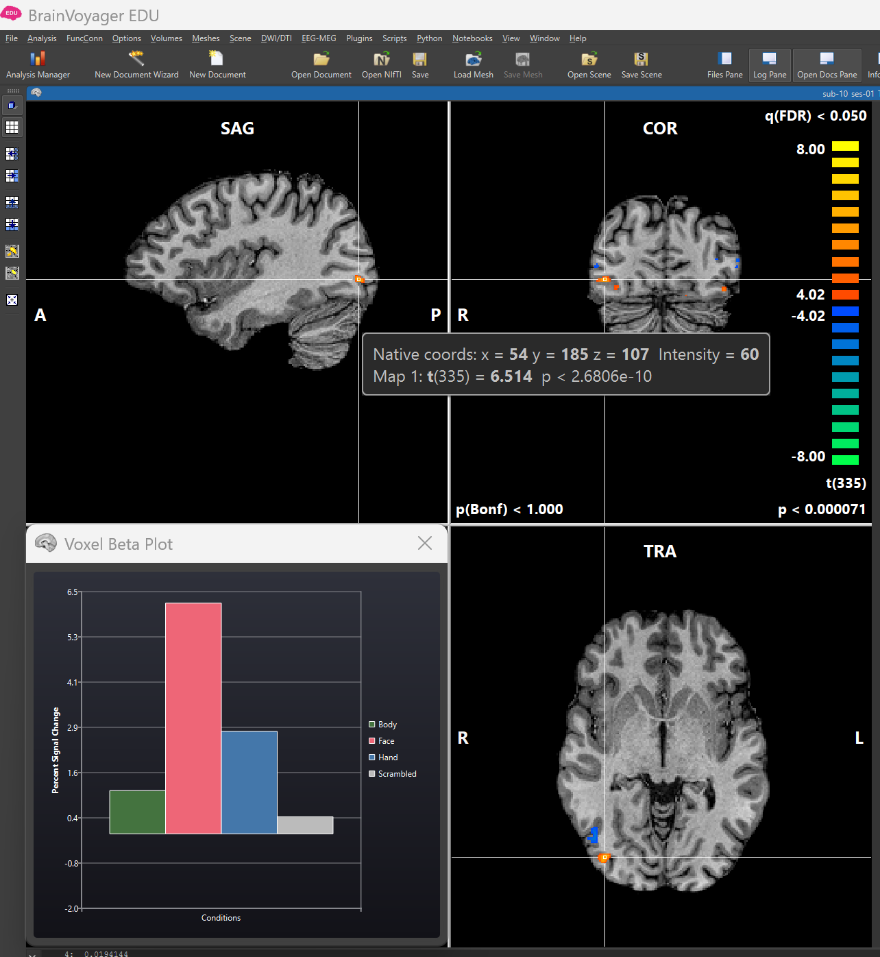
Figure 3-6. The voxel beta plot shows beta weights for a given voxel when you place the cursor over it. Beta weights are relative to the baseline = 0.
Click OK to apply the contrast. Use the mouse to move around in the brain and search for hotspots of activation. By doing this, you are specifying a hypothesis test to test whether the beta weight for Faces is significantly different (and greater than) the beta weight for Hands. This hypothesis test will be applied over all voxels, and the resulting t-statistic and p-value determine the colour intensity in the resulting heat map.
Question 6:
a) What do the numbers on the color scale on the right represent?
- The numbers represent r values.
- The numbers represent p values.
- The numbers represent t values.
- None of the above.
b) How can you interpret the colours in this heat map – does a voxel being coloured in orange-yellow vs. blue-green tell you anything about how much it activates to Faces vs Hands?
- Voxels colored in orange respond more to faces than hands while voxels colored in blue respond to images of hands to faces.
- Voxels colored in orange respond more to hands to faces while voxels colored in blue respond to images of faces than hands.
- Voxels colored in orange indicate strong activation to both faces AND hands while voxels in blue indicate zero activation to faces AND hands.
- Voxels colored in orange indicate strong activation to both faces OR hands while voxels in blue indicate zero activation to faces OR hands.
c ) Can you find any blobs that may correspond to the fusiform face area or the hand-selective region of the lateral occipitotemporal cortex?
Question 7:
a) Imagine you wanted to use contrasts to find voxels that have significantly greater activation to Faces than to Hands, Bodies and Scrambled. What are two possible contrast vectors you could use to find these voxels?
- (+3 Faces) vs (-1 Hands -1 Bodies -1 Scrambled)
- +1 Face -1 Hands -1 Bodies -1 Scrambled
- (+1 Face vs -1 Hands) AND (+1 Face vs -1 Bodies) AND (+1 Face vs -1 Scrambled)
- (+3 Face vs -1 Hands) AND (+3 Face vs -1 Bodies) AND (+3 Face vs -1 Scrambled)
b) How are these two contrasts found in question 7a different from each other?
c) Which one is more liberal and which one is stricter?