Tutorial 4 - GLM Corrections and Contrasts
Goals
Learn how to combine multiple runs from a single participant
Understand why a correction for multiple corrections is necessary. Understand the different options for correcting for multiple comparisons.
Understand the assumption that data points are independent. Understand why this is violated in fMRI data because of temporal correlations (also called serial correlations). Understand the temporal autocorrelation function can be used to check the degree to which the assumption is violated. Understand how the data can undergo a correction for serial correlations.
Understand the difference between bulk contrasts and conjunctions.
Relevant Lectures
Lecture 03c: fMRI statistics: Extending the GLM to more conditions and multiple runs
Lecture 03d: fMRI statistics: Contrasts
Lecture 03e: fMRI statistics: Corrections
Accompanying Data
Background and Overview
So far, we have done simple analyses on one run from one participant. In this tutorial, we will first learn how to extend the analysis to combine both localizer runs from the same participant. Then we will examine two statistical corrections that are necessary for fMRI data. Finally, you will compare different strategies for contrasts.
Multi-run analysis
Now that we’ve seen how to analyze one run from one participant, it’s easy to add another run. For each run, we need a volumetric functional data file (.vtc) and a single-study design matrix file (.sdm) for that run. These files can be combined in a multistudy design matrix (.mdm) .
Our participant did two runs of the Localizer, each with a different order of conditions in the protocol. Thus we need two different .sdm files.
1) Open sub-10_ses-01_T1w_BRAIN_IIHC.vmr .
2) Select Analysis/General Linear Model: Multi-Study, Multi-subject... . Once the window opens, we will add the .vtc and .sdm from run 1 and 2.
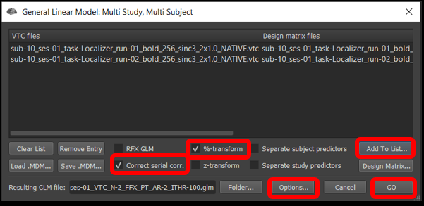
Figure 4-1. Multi-Study, Multi-Subject window
Click Add to list... , and select sub-10_ses-01_task-Localizer_run-01_bold_256_sinc3_2x1.0_NATIVE.vtc and click open , followed by sub-10_ses-01_task-Localizer_run-01_bold_256_sinc3_2x1.0_NATIVE_VTC_autosave.sdm and click open . Now, repeat this step with the files from run 2.
Make sure the %-transform and the Correct serial corr. box are checked.
Under the Options tab , click Enable mask restriction and use the Browse button beneath it to select the mask sub-10_ses-01_NATIVEBOX_vtc.msk . This is a mask that includes only functional voxels inside the brain. Click OK.
Then, click GO .
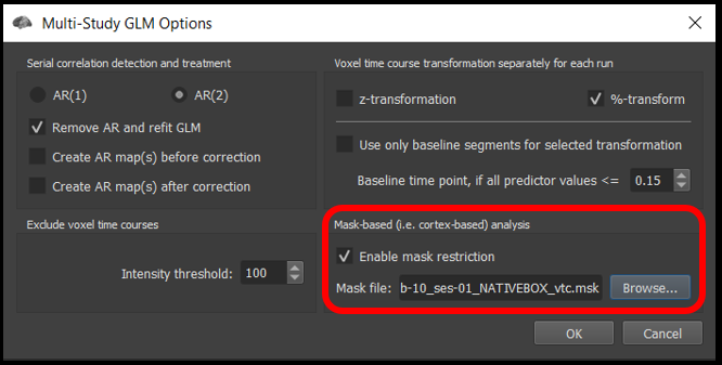
Figure 4-2. Mask restriction with this mask will only perform statistical tests on within the brain in the functional scan.
3) Select Analysis/Overlay General Linear Model..., and set the contrasts to + Faces - Hands (by default, all the prediectors will be set to [+] ). Finally, click OK .
Question 1: Complete the following sentence using the words increase and/or decrease.
Doubling the amount of data being analyzed ____ the number of df and thereby ____ your statistical power.
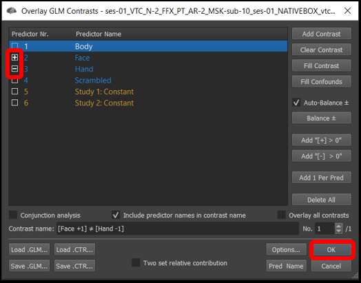
Figure 4-3. Overlay General Linear model window
Now we will look at run 1 and 2 time courses for our voxels of interest.
4) Select Analysis/Region-Of-Interest Analysis... , load the Voxels of Interest.voi file using the Load... button. Now expand the box by clicking on the < icon and add the VTCs from run 1 and 2 using the Add... button(same steps as tutorial 1).
5) Now you can select any of the six voxels and run, and visualize the time course by clicking Show Time Course.
To easily switch between the two runs, click on the green square in the bottom left corner of the time course and change in the vtc file in the section Multi-subject, mutli-run time courses. You can also show the different conditions by right clicking on the graph and selecting Show/Hide Conditions.
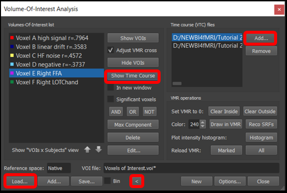
Figure 4-4. Region of interest window
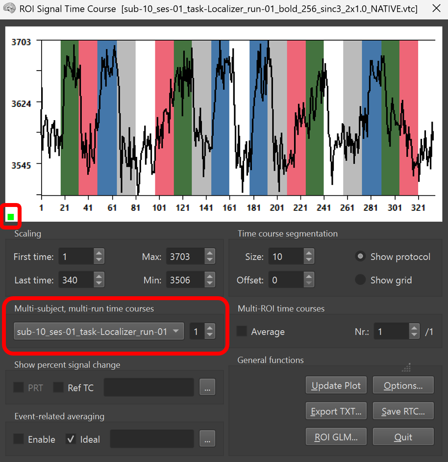
Figure 4-5. Visualizing the time course for run 1 and 2
Corrections for Multiple Comparisons
Our whole-brain voxelwise analyses have revealed which voxels are most statistically reliable, but how will we determine which p-value cut-off (threshold) to use, especially considering that the GLM was run on ~194,000 voxels. Let's explore different options.
1) Let's start with the usual convention, p < .05.
Select Analysis/Overlay volume map. Go to the Statistics tab, select Set threshold manually and uncheck Enable Cluster threshold . Then, go to the Map Options tab. Set the p-value to .05 and click Apply .

Figure 4-6. How to turn off the cluster threshold.

Figure 4-7. How to set a map threshold to a specific p value.
Question 2: Given that a p-value threshold of .05 is the usual statistical standard, why is it suboptimal for voxelwise fMRI analyses?
2) Now apply a Bonferroni correction .
Under Map Options, ensure the p value is set to .05 but this time, check the Bonferroni checkbox and click Apply .
You can see the number of voxelwise tests performed by looking in the Statistics tab, in the False Discovery Rate section.

Figure 4-8. How to see how many voxelwise tests were performed.

Question 3: For the number of voxels tested here, what is the p-value threshold? Hint: check the p value shown under the look-up table (LUT). How is it calculated?
3) Now let's look at the effects of applying a cluster correction . Generally, cluster corrections should only be used with a p-value threshold -- here called a cluster-determining threshold -- of 0.001 or stricter. Turn off Bonferroni correction and set the p-value to 0.001 . Look at the map to remember how it looks.

Figure 4-9. Example output from the cluster correction routine.
UNDER CONSTRUCTION: Jody needs to correct this. Cluster correction doesn’t work in Native space. Confirm in MNI space and specify CDT in description.We ran a plug-in in BrainVoyager to compute the likelihood of getting clusters of different sizes in 1000 randomly generated data sets where no legitimate differences between conditions were present. Here is the output: This output shows the probability of finding clusters of different sizes when no such effect is actually present (i.e., Type I errors).
Question 4: Based on this output, what is the appropriate cluster size for cluster correction? Why? Hint: Look at the alpha in the output.
In the Statistics tab, enable cluster thresholding and ensure the number of voxels matches the cutoff you determined.
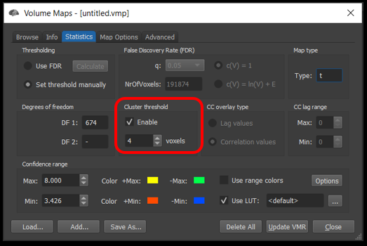
Figure 4-10. How to apply a cluster threshold.
4) Lastly, let's examine a False Discovery Rate correction. In the Statistics tab, turn on Use FDR.
Question 5: FDR uses a q value rather than a p value. Briefly and conceptually, how do q and p differ?

Figure 4-11. How to apply a False-Discovery-Rate Correction
Question 6: You've now examined the following cases: (a) uncorrected p .05; (b) Bonferroni-corrected p .05; (c) cluster threshold correction; and (d) false-discovery-rate correction. Indicate which correction approach the following pros and cons correspond to:
- Assumes independence of voxels (no clusters)
- Good approach once you have reduced the number voxels in the analysis (e.g., region of interest)
- Handicaps small regions
- High chance of finding false positives
- In most cases a good balance of Type I and Type II error
- Has low statistical power and is more vulnerable to Type II error
- Overly conservative
- Overly liberal
- Susceptible to p-hacking
- Very conservative when there is little activation
Question 7: For each of the following situations, indicate whether you must apply corrections to minimize Type I or Type II error.
- You are looking for a robust effect.
- You are analyzing a region of interest.
- Your goal is to explore data.
- You are doing a whole-brain analysis.
- You are looking for a small effect.
- You are analyzing pilot data with very few participants.
- You are conducting a confirmatory analysis, with the aim of publishing.
The problem of serial correlations
When and why serial correlations are a problem
Three things affect statistical significance, the amount of variance accounted for by the model (signal), the amount of unexplained variance (noise), and the number of data points on which the statistics are based (the degrees of freedom).
Recall from Background and Overview in Tutorial 2 that fMRI statistics can be done in two ways, based on the variability over time (if we only have data from one participant or a small number of participants, as may be the case in studies of patients or animals) or based on the variability over participants (if we have a sufficient number of participants).
Statistics assume that measurements are independent from one another. This may be easier to understand when we are considering variability over participants. For example, when doing an fMRI study, we typically want to infer that differences between conditions generalize to a population rather than just the participants we happened to sample. In such cases, we want participants to be randomly sampled from the population. In other words, we want participants to be independent from one another. The assumption of independent data points would be violated if we tested 10 participants 3 times each and treated them as independent samples instead of testing 30 different participants.
The assumption of independence also applies to the case when we are doing statistics not on multiple participants, but on one participant based on variability over time (rather than variability across participants). In this case, the number of degrees of freedom is based on number of time points.
Although the statistics assume that these sampled time points are independent of one another , this assumption violated for fMRI data. Recall that with the BOLD signal, we are not measuring neural activity directly; rather, we are measuring the effects of neural activity on regional blood oxygenation. Because blood vessels are slow to dilate and constrict, and thus the HRF is slow to rise and fall, neural activation can affect the BOLD signal for a long time (many seconds) after a neural response. Because of this, the activation in a voxel or region at one point in time is correlated with the activation for subsequent time points. This is called a serial correlation. If activation is high at one moment, it is likely to remain high for several seconds.
As such, we need to estimate how badly the assumption is violated and then we must correct for the violated assumption so that our statistical conclusions are more accurate.
How to visualize the problem of serial correlations
Sequential data points may be correlated for two reasons. First, they may be correlated because of the sequence of conditions. In our localizer run, if visual stimulation was present at one point in time, it is more likely than not that visual stimulation was also present at the next point in time. Second, they may be correlated because of temporal autocorrelations of the BOLD signal as discussed above. To evaluate the latter, we must first remove the effects of the former on the data.
One simple way to do this is to use the residuals rather than the raw time courses. Recall that the residuals are the variability over time that are “left over” once the modelled effects of conditions have been taken into account. In other words, effects due to the sequence of conditions have largely been removed from the residuals. Let’s examine the residuals for Voxel A (pink) after we have subtracted the best-fit model (green) from the data (blue).

Figure 4-12. Output of the ROI-GLM from Voxel A showing the data (blue), best-fit model (green) and residuals.

Figure 4-13. The same plot as Figure 12, showing only the residuals.
Compare the residuals from fMRI data( Figure 13) to another time series generated with a random number generator to have the same range of values (Figure 14).

Figure 4-14. A simulated residuals plot in which data points are truly random.
Question 8: How do the fMRI residuals (Figure 13) look different from random data (Figure 14)? What hints do you see from just looking that suggest there may be issues of temporal autocorrelation for fMRI data?
How can we test whether or not data have a temporal autocorrelation? One easy way is to correlate a time series with a shifted version of itself. This is called temporal autocorrelation. If the data are completely independent, the correlation for any shifts greater than 1 time point should be zero.
In the following exercise, you will generate an autocorrelation function. In Microsoft Excel or Google docs, open the spreadsheet AutocorrelationFunction.xlsx. There are two columns colored in yellow for you to fill out in order to generate the autocorrelation graph. The graph will update as you enter values in the yellow cells.
Note that the orange line shows what the data should look like if the assumption of independent samples (in this case, time points) is met.

Figure 4-15. Use this spreadsheet to plot the Autocorrelation function.
Once you have opened the spread sheet, use the widget below to compute the correlation for data that is shifted by 0 to 9 time points and enter these values into the spreadsheet to generate two new lines in the plot. Do this separately for Voxel A residuals and the randomly generated residuals.
Widget 4-1. Allows you to calculate the correlation between the original residuals function and a shifted version.
Question 9:
a) Explain why the graph of the assumption (orange line) looks like a “hockey stick”.
b) Is the assumption met for the random data? What about the fMRI data? Why or why not?
Question 10: The severity of the violation is often indicated by the the correlation for a shift of one time point, AR(1). Explain what AR(1) for the fMRI residuals indicates.
Question 11: What effect would the violation of the assumption have on your statistical significance? Why?
Voxelwise correction for serial correlations
In BrainVoyager, we can specify whether or not we want to correct for serial correlations in the voxelwise GLM.
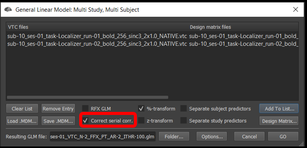
Figure 4-16. How to apply a correction for serial correlations to a voxelwise map.
Let's compare the voxelwise maps without and with a correction for serial correlations. To do this, we will compare the results from GLMs, one with and the other without correction for serial correlations. Make sure to close all previously opened windows before starting.
1) Select File/Open... and open the file sub-10_ses-01_T1w_BRAIN_IIHC.vmr .
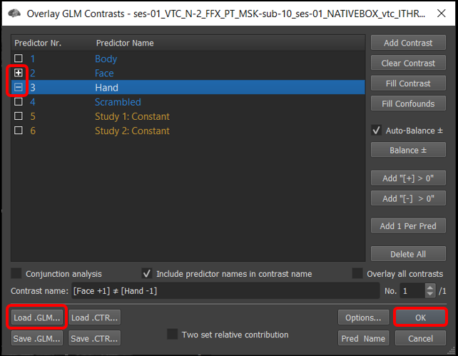
Figure 4-17. Contrast of Faces vs. Hands
2) Select Analysis/Overlay General Linear Model. Then, select Load GLM... and load ses-01_VTC_N-2_FFX_PT_MSK-sub-10_ses-01_NATIVEBOX_vtc_ITHR-100.glm. The filename doesn't include "AR-2" so we know that this is an uncorrected GLM
3) Once the GLM file is loaded, specify the contrast +Faces -Hands and click GO.
DO NOT CLOSE THIS WINDOW.
Now let's open a second window with the corrected data.
NOTE: BrainVoyager will let you have multiple windows open, even with the same VMR. However, any commands you perform will be applied to the active window. You can see the available windows by the menu bars at the top of the window. You can also select the active window using the Window menu to select the one you want. Be sure you do the next steps on the window which doesn't show any activation.
Repeat steps 1 to 3, but instead load the file ses-01_VTC_N-2_FFX_PT_AR-2_MSK-sub-10_ses-01_NATIVEBOX_vtc_ITHR-100.glm in step 2. The filename includes "AR-2" so we know that this is a corrected GLM that has corrected the data for AR-1 and AR-2
Now let's learn a useful trick in Brain Voyager for comparing maps.
4) Select Window/Tile. This will show you the two maps side by side.

Figure 4-18. The Tile function is a very useful way to compare multiple data sets (works best for an even number of data sets).
5) Click the blue box to enter blue box mode. In the blue box menu, turn on Link VMRs. Now when you move the cursor, it will show you the same location in both windows.

Figure 4-19. If you have tiled multiple windows, you can link the VMRs so that when you move the crosshairs in one VMR, the crosshairs in the VMRs will be moved to the same 3D coordinates.
6) BrainVoyager defaults to using FDR correction but this can lead to different minimum thresholds in the two images. To compare the two maps at the same threshold, for each window, Analysis/Overlay Volume Maps . Go to Statistics tab and set minimum threshold = 3 .
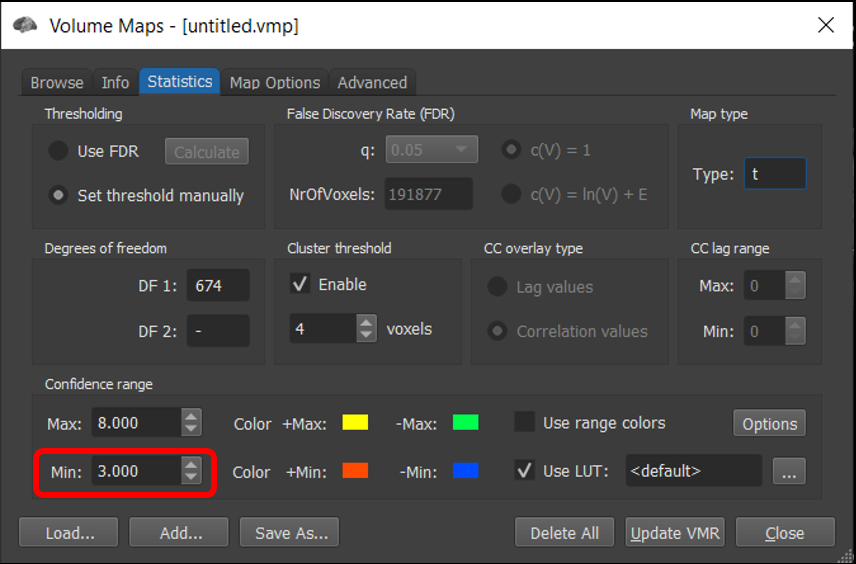
Figure 4-20. When comparing multiple maps, for a fair comparison, set the threshold to the same value in each.
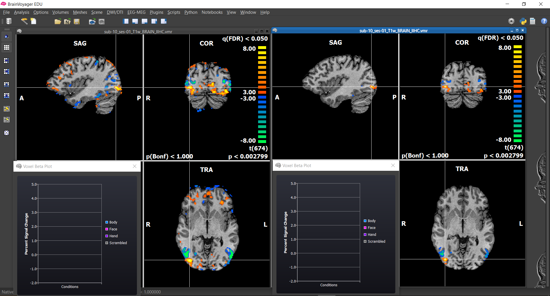
Figure 4-21. Comparison of maps without and with correction for serial correlations.
Question 12: How are the corrected and uncorrected maps different and why?
- The corrected map has less activation because the uncorrected map has decreased t-values.
- The corrected map has less activation because the uncorrected map has inflated t-values.
- The uncorrected map has more activation because the corrected map has decreased t-values.
- The uncorrected map has more activation because the corrected map has inflated t-values.
Understanding Bulk Contrast and Conjunctions
- Close one of the vmr windows you had open. In the remaining VMR window, Analysis/Overlay Volume Maps . In the Browse tab, select Load... and load the file sub-10_ses-01_run-01_Single-Bulk-Conjunction_multimap.vmp .
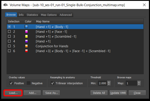
Figure 4-22. The overlap maps function can be used to store multiple voxelwise maps.
The first four maps show simple contrasts . The fifth map is a conjunction of the first four. The last map is what will call a bulk contrast .
Question 13: How can you interpret the fourth contrast Hand +1 (i.e., what is Hand activation being compared to)?
You can change which map you see by clicking on the little box [+] to the right of the map to select the one you want.
To see multiple maps superimposed, you can go to the Advanced tab and in the upper right Map Selection mode , select Multiple selections . Now when you return to the browse tab, you can put [+] before multiple maps to overlay them.

Figure 4-23. To superimpose multiple maps, you must enable Multiple selections.
Let's compare these three types of maps.
In one vmr, turn on the first three maps .
Question 14: Would the voxel at coordinates x = 43, y = 160, z = 101 be part of the conjunction? Why or why not? Would the voxel at coordinates x = 48, y = 160, z = 95 be part of the conjunction? Why or why not?
Now open a second VMR following steps 1 - 7 to tile and link VMRs. Activate the second VMR window by clicking on it; then select Analysis Overlay Volume Maps and activate the conjuntion map ( Conjunction for Hands ). Check your answers to question 14.
Select the map showing the individual contrasts and select the bulk map instead ( + Hands - Body - Face - Scrambled ).
The lateral occipitotemporal cortex contains many regions with preferred categories of visual stimuli. LOTChand shows a stronger response to hands than other categories of visual stimuli (including bodies). The extrastriate body area or EBA shows a stronger response to bodies and body parts compared to other stimuli (like chairs). These two areas are shown in Figure 24.

Figure 4-24. Bracci et al., 2010 first discovered LOTChand as an area distinct from the EBA. The crucial contrasts, areas, and beta weights are indicated in the red-outlined section
Question 15:
a) Did Bracci et al. use a bulk contrast or a conjunction?
b) Based on the contrast used to define EBA = WB + BP > H + C, can you definitively conclude any of the following individual contrasts (WB>H, WB>C, BP>H, BP>C) and thus state that the EBA responds more to bodies and body parts than other stimuli (Hint: Look at panel H of Figure 24, which corresponds to left EBA)?
Now back to our data...
Question 16:
a) Which contrast most limits the extent of activation in the conjunction? Theoretically, how could you explain this?
It can also be useful to explore the time courses of potential regions of interest to see the patterns and make sure that activation differences are not driven by noise (e.g., spikes). Find the region you think most likely to correspond to left LOTChand. Remember the data are in the radiologic convention. Move the crosshairs there, left-click to select Show ROI time course, click the green box in the lower left of the time course window to expand it, and explore the time course from the two runs.
b) In this participant's data, can you make a reasonably strong case that there is an area around the expected location of LOTChand that clearly responds more to hands than each of the other conditions? Why or why not?
c) What are some key differences between conjunctions and bulk constrasts?